Repository of Reproducible Computations

Free Statistics

of Irreproducible Research!

Author's title

Author

*Unverified author*

R Software Module

rwasp_autocorrelation.wasp

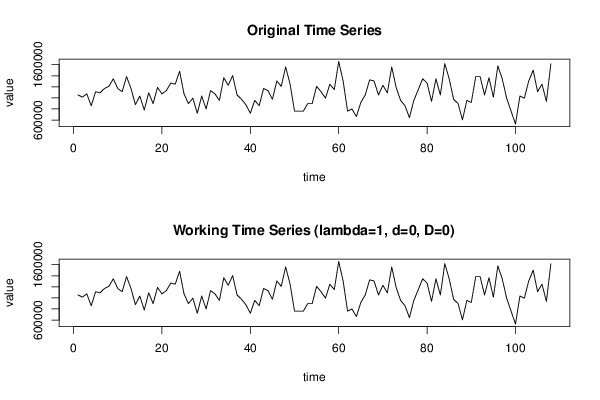
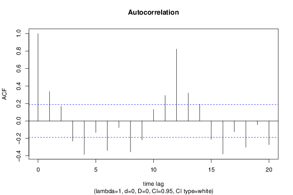
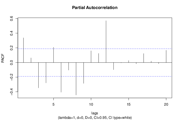
Title produced by software

(Partial) Autocorrelation Function

Date of computation

Mon, 10 Aug 2015 12:21:50 +0100

Cite this page as follows

Statistical Computations at FreeStatistics.org, Office for Research Development and Education, URL https://freestatistics.org/blog/index.php?v=date/2015/Aug/10/t1439205724xcs24j16lg1n6ri.htm/, Retrieved Sun, 19 May 2024 03:09:44 +0000

Statistical Computations at FreeStatistics.org, Office for Research Development and Education, URL https://freestatistics.org/blog/index.php?pk=279979, Retrieved Sun, 19 May 2024 03:09:44 +0000

QR Codes:

Paste this QR Code to cite your computation.

Original text written by user:

IsPrivate?

No (this computation is public)

User-defined keywords

Estimated Impact

138

Family? (F = Feedback message, R = changed R code, M = changed R Module, P = changed Parameters, D = changed Data)

-     [Histogram] [omzetontwikkeling...] [2014-09-24 09:10:11] [3d50c3f1d1505d45371c80c331b9aa00]
- R  D  [Histogram] [] [2015-07-23 12:50:11] [74be16979710d4c4e7c6647856088456]
- RMPD    [Harrell-Davis Quantiles] [] [2015-08-10 08:16:05] [74be16979710d4c4e7c6647856088456]
- RMP       [Mean versus Median] [] [2015-08-10 09:14:26] [74be16979710d4c4e7c6647856088456]
- RMP         [Mean Plot] [] [2015-08-10 09:32:31] [74be16979710d4c4e7c6647856088456]
- RMP             [(Partial) Autocorrelation Function] [] [2015-08-10 11:21:50] [d41d8cd98f00b204e9800998ecf8427e] [Current]

Feedback Forum

Post a new message

Dataseries X:

Download CSV

Histogram

Boxplots

Summary of computational transaction
Raw Input	view raw input (R code)
Raw Output	view raw output of R engine
Computing time	1 seconds
R Server	'Gwilym Jenkins' @ jenkins.wessa.net

\begin{tabular}{lllllllll}
\hline
Summary of computational transaction \tabularnewline
Raw Input & view raw input (R code)  \tabularnewline
Raw Output & view raw output of R engine  \tabularnewline
Computing time & 1 seconds \tabularnewline
R Server & 'Gwilym Jenkins' @ jenkins.wessa.net \tabularnewline
\hline
\end{tabular}
%Source: https://freestatistics.org/blog/index.php?pk=279979&T=0

[TABLE]
[ROW][C]Summary of computational transaction[/C][/ROW]
[ROW][C]Raw Input[/C][C]view raw input (R code) [/C][/ROW]
[ROW][C]Raw Output[/C][C]view raw output of R engine [/C][/ROW]
[ROW][C]Computing time[/C][C]1 seconds[/C][/ROW]
[ROW][C]R Server[/C][C]'Gwilym Jenkins' @ jenkins.wessa.net[/C][/ROW]
[/TABLE]
Source: https://freestatistics.org/blog/index.php?pk=279979&T=0

Globally Unique Identifier (entire table): ba.freestatistics.org/blog/index.php?pk=279979&T=0

As an alternative you can also use a QR Code:

The GUIDs for individual cells are displayed in the table below:

Summary of computational transaction
Raw Input	view raw input (R code)
Raw Output	view raw output of R engine
Computing time	1 seconds
R Server	'Gwilym Jenkins' @ jenkins.wessa.net

Autocorrelation Function
Time lag k	ACF(k)	T-STAT	P-value
1	0.336663	3.4987	0.00034
2	0.169057	1.7569	0.040885
3	-0.231794	-2.4089	0.008847
4	-0.382786	-3.978	6.3e-05
5	-0.131504	-1.3666	0.087291
6	-0.338556	-3.5184	0.000318
7	-0.077437	-0.8048	0.211365
8	-0.354641	-3.6855	0.000179
9	-0.217904	-2.2645	0.012769
10	0.133267	1.385	0.084461
11	0.291638	3.0308	0.001527
12	0.822222	8.5448	0
13	0.319663	3.322	0.00061
14	0.190796	1.9828	0.024964
15	-0.211977	-2.2029	0.014862
16	-0.378625	-3.9348	7.4e-05
17	-0.123426	-1.2827	0.101174
18	-0.302499	-3.1437	0.001077
19	-0.043995	-0.4572	0.324218
20	-0.271734	-2.8239	0.002825

\begin{tabular}{lllllllll}
\hline
Autocorrelation Function \tabularnewline
Time lag k & ACF(k) & T-STAT & P-value \tabularnewline
1 & 0.336663 & 3.4987 & 0.00034 \tabularnewline
2 & 0.169057 & 1.7569 & 0.040885 \tabularnewline
3 & -0.231794 & -2.4089 & 0.008847 \tabularnewline
4 & -0.382786 & -3.978 & 6.3e-05 \tabularnewline
5 & -0.131504 & -1.3666 & 0.087291 \tabularnewline
6 & -0.338556 & -3.5184 & 0.000318 \tabularnewline
7 & -0.077437 & -0.8048 & 0.211365 \tabularnewline
8 & -0.354641 & -3.6855 & 0.000179 \tabularnewline
9 & -0.217904 & -2.2645 & 0.012769 \tabularnewline
10 & 0.133267 & 1.385 & 0.084461 \tabularnewline
11 & 0.291638 & 3.0308 & 0.001527 \tabularnewline
12 & 0.822222 & 8.5448 & 0 \tabularnewline
13 & 0.319663 & 3.322 & 0.00061 \tabularnewline
14 & 0.190796 & 1.9828 & 0.024964 \tabularnewline
15 & -0.211977 & -2.2029 & 0.014862 \tabularnewline
16 & -0.378625 & -3.9348 & 7.4e-05 \tabularnewline
17 & -0.123426 & -1.2827 & 0.101174 \tabularnewline
18 & -0.302499 & -3.1437 & 0.001077 \tabularnewline
19 & -0.043995 & -0.4572 & 0.324218 \tabularnewline
20 & -0.271734 & -2.8239 & 0.002825 \tabularnewline
\hline
\end{tabular}
%Source: https://freestatistics.org/blog/index.php?pk=279979&T=1

[TABLE]
[ROW][C]Autocorrelation Function[/C][/ROW]
[ROW][C]Time lag k[/C][C]ACF(k)[/C][C]T-STAT[/C][C]P-value[/C][/ROW]
[ROW][C]1[/C][C]0.336663[/C][C]3.4987[/C][C]0.00034[/C][/ROW]
[ROW][C]2[/C][C]0.169057[/C][C]1.7569[/C][C]0.040885[/C][/ROW]
[ROW][C]3[/C][C]-0.231794[/C][C]-2.4089[/C][C]0.008847[/C][/ROW]
[ROW][C]4[/C][C]-0.382786[/C][C]-3.978[/C][C]6.3e-05[/C][/ROW]
[ROW][C]5[/C][C]-0.131504[/C][C]-1.3666[/C][C]0.087291[/C][/ROW]
[ROW][C]6[/C][C]-0.338556[/C][C]-3.5184[/C][C]0.000318[/C][/ROW]
[ROW][C]7[/C][C]-0.077437[/C][C]-0.8048[/C][C]0.211365[/C][/ROW]
[ROW][C]8[/C][C]-0.354641[/C][C]-3.6855[/C][C]0.000179[/C][/ROW]
[ROW][C]9[/C][C]-0.217904[/C][C]-2.2645[/C][C]0.012769[/C][/ROW]
[ROW][C]10[/C][C]0.133267[/C][C]1.385[/C][C]0.084461[/C][/ROW]
[ROW][C]11[/C][C]0.291638[/C][C]3.0308[/C][C]0.001527[/C][/ROW]
[ROW][C]12[/C][C]0.822222[/C][C]8.5448[/C][C]0[/C][/ROW]
[ROW][C]13[/C][C]0.319663[/C][C]3.322[/C][C]0.00061[/C][/ROW]
[ROW][C]14[/C][C]0.190796[/C][C]1.9828[/C][C]0.024964[/C][/ROW]
[ROW][C]15[/C][C]-0.211977[/C][C]-2.2029[/C][C]0.014862[/C][/ROW]
[ROW][C]16[/C][C]-0.378625[/C][C]-3.9348[/C][C]7.4e-05[/C][/ROW]
[ROW][C]17[/C][C]-0.123426[/C][C]-1.2827[/C][C]0.101174[/C][/ROW]
[ROW][C]18[/C][C]-0.302499[/C][C]-3.1437[/C][C]0.001077[/C][/ROW]
[ROW][C]19[/C][C]-0.043995[/C][C]-0.4572[/C][C]0.324218[/C][/ROW]
[ROW][C]20[/C][C]-0.271734[/C][C]-2.8239[/C][C]0.002825[/C][/ROW]
[/TABLE]
Source: https://freestatistics.org/blog/index.php?pk=279979&T=1

Globally Unique Identifier (entire table): ba.freestatistics.org/blog/index.php?pk=279979&T=1

As an alternative you can also use a QR Code:

The GUIDs for individual cells are displayed in the table below:

Autocorrelation Function
Time lag k	ACF(k)	T-STAT	P-value
1	0.336663	3.4987	0.00034
2	0.169057	1.7569	0.040885
3	-0.231794	-2.4089	0.008847
4	-0.382786	-3.978	6.3e-05
5	-0.131504	-1.3666	0.087291
6	-0.338556	-3.5184	0.000318
7	-0.077437	-0.8048	0.211365
8	-0.354641	-3.6855	0.000179
9	-0.217904	-2.2645	0.012769
10	0.133267	1.385	0.084461
11	0.291638	3.0308	0.001527
12	0.822222	8.5448	0
13	0.319663	3.322	0.00061
14	0.190796	1.9828	0.024964
15	-0.211977	-2.2029	0.014862
16	-0.378625	-3.9348	7.4e-05
17	-0.123426	-1.2827	0.101174
18	-0.302499	-3.1437	0.001077
19	-0.043995	-0.4572	0.324218
20	-0.271734	-2.8239	0.002825

Partial Autocorrelation Function
Time lag k	PACF(k)	T-STAT	P-value
1	0.336663	3.4987	0.00034
2	0.062838	0.653	0.257563
3	-0.34681	-3.6042	0.000238
4	-0.279258	-2.9021	0.002247
5	0.207078	2.152	0.016812
6	-0.405723	-4.2164	2.6e-05
7	-0.104224	-1.0831	0.140582
8	-0.444314	-4.6174	5e-06
9	-0.286191	-2.9742	0.001812
10	0.159992	1.6627	0.049637
11	0.123631	1.2848	0.100804
12	0.571132	5.9354	0
13	-0.098578	-1.0245	0.153955
14	-0.005205	-0.0541	0.47848
15	0.026664	0.2771	0.391115
16	-0.017876	-0.1858	0.426486
17	0.12199	1.2678	0.103805
18	0.01868	0.1941	0.423221
19	-0.015145	-0.1574	0.437615
20	0.166723	1.7326	0.043007

\begin{tabular}{lllllllll}
\hline
Partial Autocorrelation Function \tabularnewline
Time lag k & PACF(k) & T-STAT & P-value \tabularnewline
1 & 0.336663 & 3.4987 & 0.00034 \tabularnewline
2 & 0.062838 & 0.653 & 0.257563 \tabularnewline
3 & -0.34681 & -3.6042 & 0.000238 \tabularnewline
4 & -0.279258 & -2.9021 & 0.002247 \tabularnewline
5 & 0.207078 & 2.152 & 0.016812 \tabularnewline
6 & -0.405723 & -4.2164 & 2.6e-05 \tabularnewline
7 & -0.104224 & -1.0831 & 0.140582 \tabularnewline
8 & -0.444314 & -4.6174 & 5e-06 \tabularnewline
9 & -0.286191 & -2.9742 & 0.001812 \tabularnewline
10 & 0.159992 & 1.6627 & 0.049637 \tabularnewline
11 & 0.123631 & 1.2848 & 0.100804 \tabularnewline
12 & 0.571132 & 5.9354 & 0 \tabularnewline
13 & -0.098578 & -1.0245 & 0.153955 \tabularnewline
14 & -0.005205 & -0.0541 & 0.47848 \tabularnewline
15 & 0.026664 & 0.2771 & 0.391115 \tabularnewline
16 & -0.017876 & -0.1858 & 0.426486 \tabularnewline
17 & 0.12199 & 1.2678 & 0.103805 \tabularnewline
18 & 0.01868 & 0.1941 & 0.423221 \tabularnewline
19 & -0.015145 & -0.1574 & 0.437615 \tabularnewline
20 & 0.166723 & 1.7326 & 0.043007 \tabularnewline
\hline
\end{tabular}
%Source: https://freestatistics.org/blog/index.php?pk=279979&T=2

[TABLE]
[ROW][C]Partial Autocorrelation Function[/C][/ROW]
[ROW][C]Time lag k[/C][C]PACF(k)[/C][C]T-STAT[/C][C]P-value[/C][/ROW]
[ROW][C]1[/C][C]0.336663[/C][C]3.4987[/C][C]0.00034[/C][/ROW]
[ROW][C]2[/C][C]0.062838[/C][C]0.653[/C][C]0.257563[/C][/ROW]
[ROW][C]3[/C][C]-0.34681[/C][C]-3.6042[/C][C]0.000238[/C][/ROW]
[ROW][C]4[/C][C]-0.279258[/C][C]-2.9021[/C][C]0.002247[/C][/ROW]
[ROW][C]5[/C][C]0.207078[/C][C]2.152[/C][C]0.016812[/C][/ROW]
[ROW][C]6[/C][C]-0.405723[/C][C]-4.2164[/C][C]2.6e-05[/C][/ROW]
[ROW][C]7[/C][C]-0.104224[/C][C]-1.0831[/C][C]0.140582[/C][/ROW]
[ROW][C]8[/C][C]-0.444314[/C][C]-4.6174[/C][C]5e-06[/C][/ROW]
[ROW][C]9[/C][C]-0.286191[/C][C]-2.9742[/C][C]0.001812[/C][/ROW]
[ROW][C]10[/C][C]0.159992[/C][C]1.6627[/C][C]0.049637[/C][/ROW]
[ROW][C]11[/C][C]0.123631[/C][C]1.2848[/C][C]0.100804[/C][/ROW]
[ROW][C]12[/C][C]0.571132[/C][C]5.9354[/C][C]0[/C][/ROW]
[ROW][C]13[/C][C]-0.098578[/C][C]-1.0245[/C][C]0.153955[/C][/ROW]
[ROW][C]14[/C][C]-0.005205[/C][C]-0.0541[/C][C]0.47848[/C][/ROW]
[ROW][C]15[/C][C]0.026664[/C][C]0.2771[/C][C]0.391115[/C][/ROW]
[ROW][C]16[/C][C]-0.017876[/C][C]-0.1858[/C][C]0.426486[/C][/ROW]
[ROW][C]17[/C][C]0.12199[/C][C]1.2678[/C][C]0.103805[/C][/ROW]
[ROW][C]18[/C][C]0.01868[/C][C]0.1941[/C][C]0.423221[/C][/ROW]
[ROW][C]19[/C][C]-0.015145[/C][C]-0.1574[/C][C]0.437615[/C][/ROW]
[ROW][C]20[/C][C]0.166723[/C][C]1.7326[/C][C]0.043007[/C][/ROW]
[/TABLE]
Source: https://freestatistics.org/blog/index.php?pk=279979&T=2

Globally Unique Identifier (entire table): ba.freestatistics.org/blog/index.php?pk=279979&T=2

As an alternative you can also use a QR Code:

The GUIDs for individual cells are displayed in the table below:

Partial Autocorrelation Function
Time lag k	PACF(k)	T-STAT	P-value
1	0.336663	3.4987	0.00034
2	0.062838	0.653	0.257563
3	-0.34681	-3.6042	0.000238
4	-0.279258	-2.9021	0.002247
5	0.207078	2.152	0.016812
6	-0.405723	-4.2164	2.6e-05
7	-0.104224	-1.0831	0.140582
8	-0.444314	-4.6174	5e-06
9	-0.286191	-2.9742	0.001812
10	0.159992	1.6627	0.049637
11	0.123631	1.2848	0.100804
12	0.571132	5.9354	0
13	-0.098578	-1.0245	0.153955
14	-0.005205	-0.0541	0.47848
15	0.026664	0.2771	0.391115
16	-0.017876	-0.1858	0.426486
17	0.12199	1.2678	0.103805
18	0.01868	0.1941	0.423221
19	-0.015145	-0.1574	0.437615
20	0.166723	1.7326	0.043007

Figure 1

PNG link

Postscript link

PDF link

Figure 2

PNG link

Postscript link

PDF link

Figure 3

PNG link

Postscript link

PDF link

Parameters (Session):

par1 = Default ; par2 = 1 ; par3 = 0 ; par4 = 0 ; par5 = 12 ; par6 = White Noise ; par7 = 0.95 ;

Parameters (R input):

par1 = Default ; par2 = 1 ; par3 = 0 ; par4 = 0 ; par5 = 12 ; par6 = White Noise ; par7 = 0.95 ; par8 = ;

R code (references can be found in the software module):

if (par1 == 'Default') {
par1 = 10*log10(length(x))
} else {
par1 <- as.numeric(par1)
}
par2 <- as.numeric(par2)
par3 <- as.numeric(par3)
par4 <- as.numeric(par4)
par5 <- as.numeric(par5)
if (par6 == 'White Noise') par6 <- 'white' else par6 <- 'ma'
par7 <- as.numeric(par7)
if (par8 != '') par8 <- as.numeric(par8)
ox <- x
if (par8 == '') {
if (par2 == 0) {
x <- log(x)
} else {
x <- (x ^ par2 - 1) / par2
}
} else {
x <- log(x,base=par8)
}
if (par3 > 0) x <- diff(x,lag=1,difference=par3)
if (par4 > 0) x <- diff(x,lag=par5,difference=par4)
bitmap(file='picts.png')
op <- par(mfrow=c(2,1))
plot(ox,type='l',main='Original Time Series',xlab='time',ylab='value')
if (par8=='') {
mytitle <- paste('Working Time Series (lambda=',par2,', d=',par3,', D=',par4,')',sep='')
mysub <- paste('(lambda=',par2,', d=',par3,', D=',par4,', CI=', par7, ', CI type=',par6,')',sep='')
} else {
mytitle <- paste('Working Time Series (base=',par8,', d=',par3,', D=',par4,')',sep='')
mysub <- paste('(base=',par8,', d=',par3,', D=',par4,', CI=', par7, ', CI type=',par6,')',sep='')
}
plot(x,type='l', main=mytitle,xlab='time',ylab='value')
par(op)
dev.off()
bitmap(file='pic1.png')
racf <- acf(x, par1, main='Autocorrelation', xlab='time lag', ylab='ACF', ci.type=par6, ci=par7, sub=mysub)
dev.off()
bitmap(file='pic2.png')
rpacf <- pacf(x,par1,main='Partial Autocorrelation',xlab='lags',ylab='PACF',sub=mysub)
dev.off()
(myacf <- c(racf$acf))
(mypacf <- c(rpacf$acf))
lengthx <- length(x)
sqrtn <- sqrt(lengthx)
load(file='createtable')
a<-table.start()
a<-table.row.start(a)
a<-table.element(a,'Autocorrelation Function',4,TRUE)
a<-table.row.end(a)
a<-table.row.start(a)
a<-table.element(a,'Time lag k',header=TRUE)
a<-table.element(a,hyperlink('basics.htm','ACF(k)','click here for more information about the Autocorrelation Function'),header=TRUE)
a<-table.element(a,'T-STAT',header=TRUE)
a<-table.element(a,'P-value',header=TRUE)
a<-table.row.end(a)
for (i in 2:(par1+1)) {
a<-table.row.start(a)
a<-table.element(a,i-1,header=TRUE)
a<-table.element(a,round(myacf[i],6))
mytstat <- myacf[i]*sqrtn
a<-table.element(a,round(mytstat,4))
a<-table.element(a,round(1-pt(abs(mytstat),lengthx),6))
a<-table.row.end(a)
}
a<-table.end(a)
table.save(a,file='mytable.tab')
a<-table.start()
a<-table.row.start(a)
a<-table.element(a,'Partial Autocorrelation Function',4,TRUE)
a<-table.row.end(a)
a<-table.row.start(a)
a<-table.element(a,'Time lag k',header=TRUE)
a<-table.element(a,hyperlink('basics.htm','PACF(k)','click here for more information about the Partial Autocorrelation Function'),header=TRUE)
a<-table.element(a,'T-STAT',header=TRUE)
a<-table.element(a,'P-value',header=TRUE)
a<-table.row.end(a)
for (i in 1:par1) {
a<-table.row.start(a)
a<-table.element(a,i,header=TRUE)
a<-table.element(a,round(mypacf[i],6))
mytstat <- mypacf[i]*sqrtn
a<-table.element(a,round(mytstat,4))
a<-table.element(a,round(1-pt(abs(mytstat),lengthx),6))
a<-table.row.end(a)
}
a<-table.end(a)
table.save(a,file='mytable1.tab')

Free Statistics

Description of Statistical Computation

Tree of Dependent Computations

Dataset

Tables (Output of Computation)

Figures (Output of Computation)

Input Parameters & R Code