Free Statistics
of Irreproducible Research!
Description of Statistical Computation | |||||||||||||||||||||
|---|---|---|---|---|---|---|---|---|---|---|---|---|---|---|---|---|---|---|---|---|---|
| Author's title | |||||||||||||||||||||
| Author | *Unverified author* | ||||||||||||||||||||
| R Software Module | rwasp_meanplot.wasp | ||||||||||||||||||||
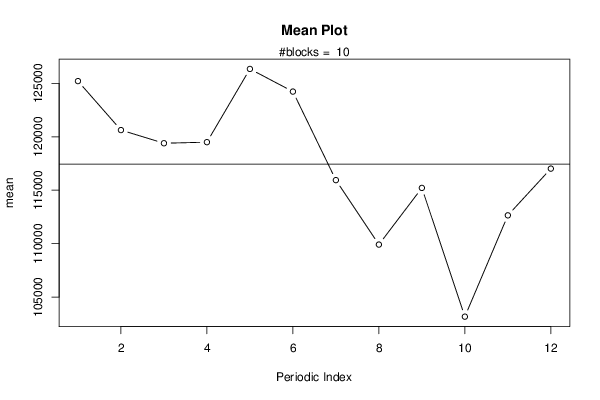
| Title produced by software | Mean Plot | ||||||||||||||||||||
| Date of computation | Sat, 15 Aug 2015 16:36:46 +0100 | ||||||||||||||||||||
| Cite this page as follows | Statistical Computations at FreeStatistics.org, Office for Research Development and Education, URL https://freestatistics.org/blog/index.php?v=date/2015/Aug/15/t143965305364fa2bm9x4drbrc.htm/, Retrieved Wed, 15 May 2024 09:00:17 +0000 | ||||||||||||||||||||
| Statistical Computations at FreeStatistics.org, Office for Research Development and Education, URL https://freestatistics.org/blog/index.php?pk=280099, Retrieved Wed, 15 May 2024 09:00:17 +0000 | |||||||||||||||||||||
| QR Codes: | |||||||||||||||||||||
|
| |||||||||||||||||||||
| Original text written by user: | |||||||||||||||||||||
| IsPrivate? | No (this computation is public) | ||||||||||||||||||||
| User-defined keywords | |||||||||||||||||||||
| Estimated Impact | 120 | ||||||||||||||||||||
Tree of Dependent Computations | |||||||||||||||||||||
| Family? (F = Feedback message, R = changed R code, M = changed R Module, P = changed Parameters, D = changed Data) | |||||||||||||||||||||
| - [Mean Plot] [Mean plot voor om...] [2015-08-15 15:36:46] [0d8529ada52922935dd1fcf0fb375c74] [Current] | |||||||||||||||||||||
| Feedback Forum | |||||||||||||||||||||
Post a new message | |||||||||||||||||||||
Dataset | |||||||||||||||||||||
| Dataseries X: | |||||||||||||||||||||
133448,00 132951,00 132447,00 131404,00 141722,00 141176,00 133448,00 128310,00 128807,00 128807,00 129360,00 130354,00 131901,00 131901,00 130907,00 128310,00 141722,00 143766,00 140679,00 133448,00 136542,00 131901,00 133994,00 134995,00 136038,00 133448,00 133994,00 130354,00 141722,00 145313,00 142226,00 136542,00 142723,00 136038,00 142226,00 141722,00 143269,00 137585,00 143766,00 143269,00 152544,00 150451,00 142226,00 138082,00 143766,00 136038,00 141722,00 142723,00 144816,00 140182,00 142723,00 144270,00 149954,00 145313,00 139132,00 132447,00 138635,00 121625,00 129857,00 134491,00 139132,00 132447,00 132447,00 132447,00 136038,00 130907,00 124173,00 118538,00 122626,00 106666,00 116445,00 122129,00 123172,00 117488,00 117985,00 116445,00 121625,00 117985,00 110810,00 105623,00 114394,00 95347,00 107716,00 113351,00 113351,00 106666,00 100485,00 99988,00 105623,00 100485,00 90713,00 83979,00 91210,00 74207,00 89663,00 97888,00 100485,00 94801,00 87619,00 92757,00 94801,00 93254,00 77791,00 70616,00 75747,00 60291,00 76251,00 81935,00 86569,00 78841,00 71610,00 75747,00 77791,00 73703,00 58247,00 51513,00 57694,00 40691,00 59241,00 70616,00 | |||||||||||||||||||||
Tables (Output of Computation) | |||||||||||||||||||||
| |||||||||||||||||||||
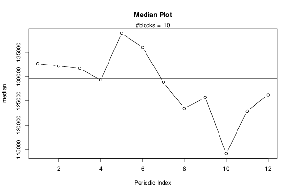
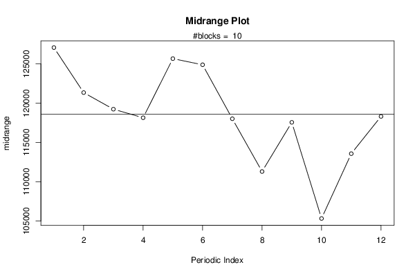
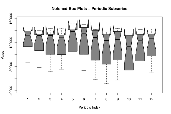
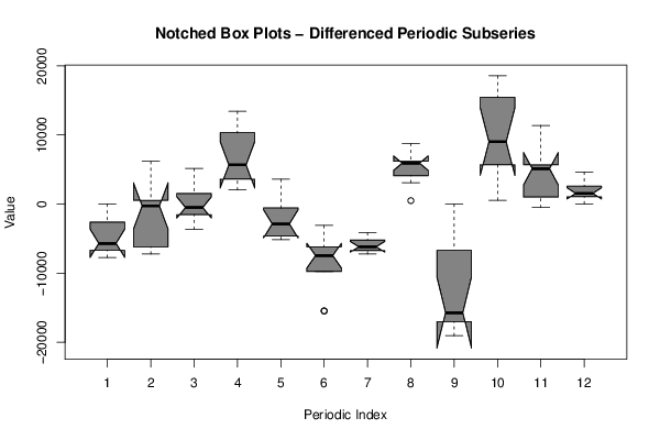
Figures (Output of Computation) | |||||||||||||||||||||
Input Parameters & R Code | |||||||||||||||||||||
| Parameters (Session): | |||||||||||||||||||||
| par1 = 12 ; | |||||||||||||||||||||
| Parameters (R input): | |||||||||||||||||||||
| par1 = 12 ; | |||||||||||||||||||||
| R code (references can be found in the software module): | |||||||||||||||||||||
par1 <- as.numeric(par1) | |||||||||||||||||||||