Repository of Reproducible Computations

Free Statistics

of Irreproducible Research!

Author's title

Author

*The author of this computation has been verified*

R Software Module

rwasp_bidensity.wasp

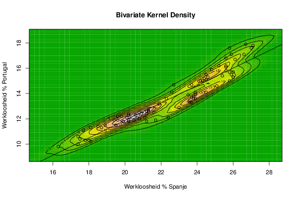
Title produced by software

Bivariate Kernel Density Estimation

Date of computation

Tue, 08 Dec 2015 20:14:32 +0000

Cite this page as follows

Statistical Computations at FreeStatistics.org, Office for Research Development and Education, URL https://freestatistics.org/blog/index.php?v=date/2015/Dec/08/t1449605709sqzve0qfxqvut0n.htm/, Retrieved Thu, 16 May 2024 15:50:18 +0000

Statistical Computations at FreeStatistics.org, Office for Research Development and Education, URL https://freestatistics.org/blog/index.php?pk=285561, Retrieved Thu, 16 May 2024 15:50:18 +0000

QR Codes:

Paste this QR Code to cite your computation.

Original text written by user:

IsPrivate?

No (this computation is public)

User-defined keywords

Estimated Impact

111

Family? (F = Feedback message, R = changed R code, M = changed R Module, P = changed Parameters, D = changed Data)

-     [One Sample Tests about the Mean] [] [2015-09-17 17:14:23] [32b17a345b130fdf5cc88718ed94a974]
- RMPD    [Bivariate Kernel Density Estimation] [Kernel Density Sp...] [2015-12-08 20:14:32] [0e991996cbbd17b3741fb533250e72dd] [Current]
- RM D      [Tukey lambda PPCC Plot] [Verdeling cijfers...] [2015-12-08 20:39:14] [08054cfd69be47a1043f60b064067192] 
- R  D        [Tukey lambda PPCC Plot] [Verdeling cijfers...] [2015-12-08 21:10:03] [08054cfd69be47a1043f60b064067192] 
- RM D        [Pearson Correlation] [Pearson Correlation] [2015-12-08 21:27:11] [08054cfd69be47a1043f60b064067192] 
- R             [Pearson Correlation] [Pearson Correlation] [2015-12-08 21:34:10] [08054cfd69be47a1043f60b064067192] 
- RM D          [Notched Boxplots] [Notched Boxplot] [2015-12-08 21:46:09] [08054cfd69be47a1043f60b064067192] 

Feedback Forum

Post a new message

Dataseries X:

Download CSV

Histogram

Boxplots

16.3
17.4
18.1
18.0
17.8
17.5
17.4
17.7
18.1
18.5
18.7
18.9
19.5
19.9
20.2
20.2
19.9
19.6
19.4
19.6
19.8
20.1
20.2
20.2
20.8
21.2
21.3
20.9
20.6
20.5
20.8
21.3
21.9
22.3
22.6
22.7
23.7
24.3
24.6
24.5
24.5
24.2
24.4
24.8
25.2
25.6
25.9
25.8
26.7
27.1
27.0
26.6
26.1
25.6
25.6
25.6
25.8
26.0
25.9
25.4
26.0
26.0
25.8
25.1
24.5
23.8
23.7
23.6
23.7
23.9
23.8
23.5
23.9
23.9
23.6
23.0
22.4
21.7
21.2
21.1
21.2
21.6

Dataseries Y:

Download CSV

Histogram

9.8
10.0
10.2
10.3
10.3
10.4
10.6
11.1
11.3
11.4
11.3
11.5
11.5
11.8
11.8
11.9
11.8
11.9
11.9
12.2
12.2
12.1
12.3
12.4
12.5
12.6
12.7
12.4
12.3
11.9
12.0
12.6
13.2
13.6
14.1
14.7
14.7
15.0
15.3
15.5
15.1
15.0
15.2
15.9
16.2
16.8
17.1
17.6
17.9
17.8
17.6
17.1
16.7
16.1
16.2
15.8
15.7
15.7
15.5
15.4
15.3
15.3
15.0
14.6
14.1
13.8
13.7
13.3
13.3
13.6
13.6
13.9
14.1
13.9
13.4
12.9
12.1
11.9
11.8
12.1
12.4
12.5

Summary of computational transaction
Raw Input	view raw input (R code)
Raw Output	view raw output of R engine
Computing time	1 seconds
R Server	'Sir Maurice George Kendall' @ kendall.wessa.net

\begin{tabular}{lllllllll}
\hline
Summary of computational transaction \tabularnewline
Raw Input & view raw input (R code)  \tabularnewline
Raw Output & view raw output of R engine  \tabularnewline
Computing time & 1 seconds \tabularnewline
R Server & 'Sir Maurice George Kendall' @ kendall.wessa.net \tabularnewline
\hline
\end{tabular}
%Source: https://freestatistics.org/blog/index.php?pk=285561&T=0

[TABLE]
[ROW][C]Summary of computational transaction[/C][/ROW]
[ROW][C]Raw Input[/C][C]view raw input (R code) [/C][/ROW]
[ROW][C]Raw Output[/C][C]view raw output of R engine [/C][/ROW]
[ROW][C]Computing time[/C][C]1 seconds[/C][/ROW]
[ROW][C]R Server[/C][C]'Sir Maurice George Kendall' @ kendall.wessa.net[/C][/ROW]
[/TABLE]
Source: https://freestatistics.org/blog/index.php?pk=285561&T=0

Globally Unique Identifier (entire table): ba.freestatistics.org/blog/index.php?pk=285561&T=0

As an alternative you can also use a QR Code:

The GUIDs for individual cells are displayed in the table below:

Summary of computational transaction
Raw Input	view raw input (R code)
Raw Output	view raw output of R engine
Computing time	1 seconds
R Server	'Sir Maurice George Kendall' @ kendall.wessa.net

Bandwidth
x axis	0.980162685108344
y axis	0.72236538831722
Correlation
correlation used in KDE	0.950886148406473
correlation(x,y)	0.950886148406473

\begin{tabular}{lllllllll}
\hline
Bandwidth \tabularnewline
x axis & 0.980162685108344 \tabularnewline
y axis & 0.72236538831722 \tabularnewline
Correlation \tabularnewline
correlation used in KDE & 0.950886148406473 \tabularnewline
correlation(x,y) & 0.950886148406473 \tabularnewline
\hline
\end{tabular}
%Source: https://freestatistics.org/blog/index.php?pk=285561&T=1

[TABLE]
[ROW][C]Bandwidth[/C][/ROW]
[ROW][C]x axis[/C][C]0.980162685108344[/C][/ROW]
[ROW][C]y axis[/C][C]0.72236538831722[/C][/ROW]
[ROW][C]Correlation[/C][/ROW]
[ROW][C]correlation used in KDE[/C][C]0.950886148406473[/C][/ROW]
[ROW][C]correlation(x,y)[/C][C]0.950886148406473[/C][/ROW]
[/TABLE]
Source: https://freestatistics.org/blog/index.php?pk=285561&T=1

Globally Unique Identifier (entire table): ba.freestatistics.org/blog/index.php?pk=285561&T=1

As an alternative you can also use a QR Code:

The GUIDs for individual cells are displayed in the table below:

Bandwidth
x axis	0.980162685108344
y axis	0.72236538831722
Correlation
correlation used in KDE	0.950886148406473
correlation(x,y)	0.950886148406473

Figure 1

PNG link

Postscript link

PDF link

Parameters (Session):

par1 = grey ;

Parameters (R input):

par1 = 50 ; par2 = 50 ; par3 = 0 ; par4 = 0 ; par5 = 0 ; par6 = Y ; par7 = Y ; par8 = terrain.colors ;

R code (references can be found in the software module):

par8 <- 'terrain.colors'
par7 <- 'Y'
par6 <- 'Y'
par5 <- '0'
par4 <- '0'
par3 <- '0'
par2 <- '50'
par1 <- '50'
par1 <- as(par1,'numeric')
par2 <- as(par2,'numeric')
par3 <- as(par3,'numeric')
par4 <- as(par4,'numeric')
par5 <- as(par5,'numeric')
library('GenKern')
x <- x[!is.na(y)]
y <- y[!is.na(y)]
y <- y[!is.na(x)]
x <- x[!is.na(x)]
if (par3==0) par3 <- dpik(x)
if (par4==0) par4 <- dpik(y)
if (par5==0) par5 <- cor(x,y)
if (par1 > 500) par1 <- 500
if (par2 > 500) par2 <- 500
if (par8 == 'terrain.colors') mycol <- terrain.colors(100)
if (par8 == 'rainbow') mycol <- rainbow(100)
if (par8 == 'heat.colors') mycol <- heat.colors(100)
if (par8 == 'topo.colors') mycol <- topo.colors(100)
if (par8 == 'cm.colors') mycol <- cm.colors(100)
bitmap(file='bidensity.png')
op <- KernSur(x,y, xgridsize=par1, ygridsize=par2, correlation=par5, xbandwidth=par3, ybandwidth=par4)
image(op$xords, op$yords, op$zden, col=mycol, axes=TRUE,main=main,xlab=xlab,ylab=ylab)
if (par6=='Y') contour(op$xords, op$yords, op$zden, add=TRUE)
if (par7=='Y') points(x,y)
(r<-lm(y ~ x))
abline(r)
box()
dev.off()
load(file='createtable')
a<-table.start()
a<-table.row.start(a)
a<-table.element(a,'Bandwidth',2,TRUE)
a<-table.row.end(a)
a<-table.row.start(a)
a<-table.element(a,'x axis',header=TRUE)
a<-table.element(a,par3)
a<-table.row.end(a)
a<-table.row.start(a)
a<-table.element(a,'y axis',header=TRUE)
a<-table.element(a,par4)
a<-table.row.end(a)
a<-table.row.start(a)
a<-table.element(a,'Correlation',2,TRUE)
a<-table.row.end(a)
a<-table.row.start(a)
a<-table.element(a,'correlation used in KDE',header=TRUE)
a<-table.element(a,par5)
a<-table.row.end(a)
a<-table.row.start(a)
a<-table.element(a,'correlation(x,y)',header=TRUE)
a<-table.element(a,cor(x,y))
a<-table.row.end(a)
a<-table.end(a)
table.save(a,file='mytable.tab')

Free Statistics

Description of Statistical Computation

Tree of Dependent Computations

Dataset

Tables (Output of Computation)

Figures (Output of Computation)

Input Parameters & R Code