Repository of Reproducible Computations

Free Statistics

of Irreproducible Research!

Author's title

Author

*The author of this computation has been verified*

R Software Module

rwasp_decompose.wasp

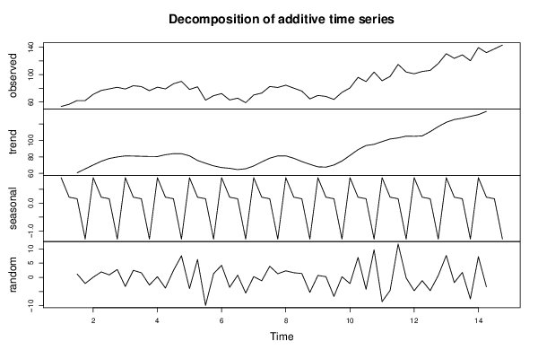
Title produced by software

Classical Decomposition

Date of computation

Wed, 09 Dec 2015 14:13:43 +0000

Cite this page as follows

Statistical Computations at FreeStatistics.org, Office for Research Development and Education, URL https://freestatistics.org/blog/index.php?v=date/2015/Dec/09/t1449670540r8vfhc6houjd82g.htm/, Retrieved Thu, 16 May 2024 23:50:34 +0000

Statistical Computations at FreeStatistics.org, Office for Research Development and Education, URL https://freestatistics.org/blog/index.php?pk=285693, Retrieved Thu, 16 May 2024 23:50:34 +0000

QR Codes:

Paste this QR Code to cite your computation.

Original text written by user:

spaargelden

IsPrivate?

No (this computation is public)

User-defined keywords

Estimated Impact

Family? (F = Feedback message, R = changed R code, M = changed R Module, P = changed Parameters, D = changed Data)

-       [Classical Decomposition] [Klassieke decompo...] [2015-12-09 14:13:43] [0699448209a825438cb2d76a05e8a0a6] [Current]

Feedback Forum

Post a new message

Dataseries X:

Download CSV

Histogram

Boxplots

Summary of computational transaction
Raw Input	view raw input (R code)
Raw Output	view raw output of R engine
Computing time	2 seconds
R Server	'Gwilym Jenkins' @ jenkins.wessa.net

\begin{tabular}{lllllllll}
\hline
Summary of computational transaction \tabularnewline
Raw Input & view raw input (R code)  \tabularnewline
Raw Output & view raw output of R engine  \tabularnewline
Computing time & 2 seconds \tabularnewline
R Server & 'Gwilym Jenkins' @ jenkins.wessa.net \tabularnewline
\hline
\end{tabular}
%Source: https://freestatistics.org/blog/index.php?pk=285693&T=0

[TABLE]
[ROW][C]Summary of computational transaction[/C][/ROW]
[ROW][C]Raw Input[/C][C]view raw input (R code) [/C][/ROW]
[ROW][C]Raw Output[/C][C]view raw output of R engine [/C][/ROW]
[ROW][C]Computing time[/C][C]2 seconds[/C][/ROW]
[ROW][C]R Server[/C][C]'Gwilym Jenkins' @ jenkins.wessa.net[/C][/ROW]
[/TABLE]
Source: https://freestatistics.org/blog/index.php?pk=285693&T=0

Globally Unique Identifier (entire table): ba.freestatistics.org/blog/index.php?pk=285693&T=0

As an alternative you can also use a QR Code:

The GUIDs for individual cells are displayed in the table below:

Summary of computational transaction
Raw Input	view raw input (R code)
Raw Output	view raw output of R engine
Computing time	2 seconds
R Server	'Gwilym Jenkins' @ jenkins.wessa.net

Classical Decomposition by Moving Averages
t	Observations	Fit	Trend	Seasonal	Random
1	53.361	NA	NA	0.910207	NA
2	56.628	NA	NA	0.2132	NA
3	62.073	60.9133	60.7548	0.158508	1.15968
4	62.073	64.2237	65.5056	-1.28192	-2.15068
5	71.1295	71.0814	70.1712	0.910207	0.0480739
6	76.86575	74.943	74.7298	0.2132	1.92271
7	79.16025	78.291	78.1325	0.158508	0.869242
8	81.45475	78.6917	79.9736	-1.28192	2.76307
9	78.969	82.1697	81.2595	0.910207	-3.20074
10	83.755	81.2877	81.0745	0.2132	2.46733
11	82.5585	80.9531	80.7946	0.158508	1.60537
12	76.576	79.2653	80.5472	-1.28192	-2.68933
13	81.609	81.3796	80.4694	0.910207	0.229355
14	79.136	82.8933	82.6801	0.2132	-3.75726
15	86.555	84.1379	83.9794	0.158508	2.41712
16	90.2645	82.6726	83.9545	-1.28192	7.59195
17	78.315	82.2636	81.3534	0.910207	-3.94864
18	82.23075	75.943	75.7298	0.2132	6.28777
19	62.652	72.4946	72.3361	0.158508	-9.84263
20	69.17825	67.8782	69.1602	-1.28192	1.30001
21	72.252	68.016	67.1058	0.910207	4.23598
22	62.886	66.3945	66.1813	0.2132	-3.50848
23	65.562	64.7968	64.6383	0.158508	0.765211
24	58.872	64.3619	65.6438	-1.28192	-5.48987
25	70.21425	69.9446	69.0344	0.910207	0.269668
26	72.96775	74.1725	73.9593	0.2132	-1.20473
27	82.605	78.7002	78.5417	0.158508	3.90477
28	81.22825	79.9542	81.2362	-1.28192	1.27401
29	84.5175	82.2176	81.3074	0.910207	2.29992
30	80.22	78.5895	78.3763	0.2132	1.63046
31	75.9225	74.5694	74.4109	0.158508	1.35305
32	64.4625	69.7418	71.0238	-1.28192	-5.27933
33	69.56	68.8811	67.9709	0.910207	0.678855
34	68.08	67.841	67.6278	0.2132	0.238987
35	63.64	70.352	70.1935	0.158508	-6.71201
36	74	73.7798	75.0618	-1.28192	0.220165
37	80.548	82.742	81.8318	0.910207	-2.19396
38	96.038	89.0431	88.8299	0.2132	6.99492
39	89.842	94.0232	93.8647	0.158508	-4.18116
40	103.783	94.0689	95.3508	-1.28192	9.71407
41	91.04325	99.5803	98.6701	0.910207	-8.53708
42	97.43225	102.033	101.82	0.2132	-4.60086
43	115.002	103.266	103.108	0.158508	11.736
44	103.82125	104.008	105.29	-1.28192	-0.186522
45	101.30575	106.01	105.1	0.910207	-4.70427
46	104.62725	105.778	105.564	0.2132	-1.15042
47	106.288	110.954	110.795	0.158508	-4.66566
48	116.2525	115.592	116.874	-1.28192	0.660884
49	130.72	123.024	122.114	0.910207	7.69567
50	123.84	125.685	125.472	0.2132	-1.84476
51	129	127.258	127.099	0.158508	1.74237
52	120.4	127.977	129.259	-1.28192	-7.57708
53	139.593	132.314	131.404	0.910207	7.27851
54	132.246	135.57	135.357	0.2132	-3.32433
55	137.75625	NA	NA	0.158508	NA
56	143.2665	NA	NA	-1.28192	NA

\begin{tabular}{lllllllll}
\hline
Classical Decomposition by Moving Averages \tabularnewline
t & Observations & Fit & Trend & Seasonal & Random \tabularnewline
1 & 53.361 & NA & NA & 0.910207 & NA \tabularnewline
2 & 56.628 & NA & NA & 0.2132 & NA \tabularnewline
3 & 62.073 & 60.9133 & 60.7548 & 0.158508 & 1.15968 \tabularnewline
4 & 62.073 & 64.2237 & 65.5056 & -1.28192 & -2.15068 \tabularnewline
5 & 71.1295 & 71.0814 & 70.1712 & 0.910207 & 0.0480739 \tabularnewline
6 & 76.86575 & 74.943 & 74.7298 & 0.2132 & 1.92271 \tabularnewline
7 & 79.16025 & 78.291 & 78.1325 & 0.158508 & 0.869242 \tabularnewline
8 & 81.45475 & 78.6917 & 79.9736 & -1.28192 & 2.76307 \tabularnewline
9 & 78.969 & 82.1697 & 81.2595 & 0.910207 & -3.20074 \tabularnewline
10 & 83.755 & 81.2877 & 81.0745 & 0.2132 & 2.46733 \tabularnewline
11 & 82.5585 & 80.9531 & 80.7946 & 0.158508 & 1.60537 \tabularnewline
12 & 76.576 & 79.2653 & 80.5472 & -1.28192 & -2.68933 \tabularnewline
13 & 81.609 & 81.3796 & 80.4694 & 0.910207 & 0.229355 \tabularnewline
14 & 79.136 & 82.8933 & 82.6801 & 0.2132 & -3.75726 \tabularnewline
15 & 86.555 & 84.1379 & 83.9794 & 0.158508 & 2.41712 \tabularnewline
16 & 90.2645 & 82.6726 & 83.9545 & -1.28192 & 7.59195 \tabularnewline
17 & 78.315 & 82.2636 & 81.3534 & 0.910207 & -3.94864 \tabularnewline
18 & 82.23075 & 75.943 & 75.7298 & 0.2132 & 6.28777 \tabularnewline
19 & 62.652 & 72.4946 & 72.3361 & 0.158508 & -9.84263 \tabularnewline
20 & 69.17825 & 67.8782 & 69.1602 & -1.28192 & 1.30001 \tabularnewline
21 & 72.252 & 68.016 & 67.1058 & 0.910207 & 4.23598 \tabularnewline
22 & 62.886 & 66.3945 & 66.1813 & 0.2132 & -3.50848 \tabularnewline
23 & 65.562 & 64.7968 & 64.6383 & 0.158508 & 0.765211 \tabularnewline
24 & 58.872 & 64.3619 & 65.6438 & -1.28192 & -5.48987 \tabularnewline
25 & 70.21425 & 69.9446 & 69.0344 & 0.910207 & 0.269668 \tabularnewline
26 & 72.96775 & 74.1725 & 73.9593 & 0.2132 & -1.20473 \tabularnewline
27 & 82.605 & 78.7002 & 78.5417 & 0.158508 & 3.90477 \tabularnewline
28 & 81.22825 & 79.9542 & 81.2362 & -1.28192 & 1.27401 \tabularnewline
29 & 84.5175 & 82.2176 & 81.3074 & 0.910207 & 2.29992 \tabularnewline
30 & 80.22 & 78.5895 & 78.3763 & 0.2132 & 1.63046 \tabularnewline
31 & 75.9225 & 74.5694 & 74.4109 & 0.158508 & 1.35305 \tabularnewline
32 & 64.4625 & 69.7418 & 71.0238 & -1.28192 & -5.27933 \tabularnewline
33 & 69.56 & 68.8811 & 67.9709 & 0.910207 & 0.678855 \tabularnewline
34 & 68.08 & 67.841 & 67.6278 & 0.2132 & 0.238987 \tabularnewline
35 & 63.64 & 70.352 & 70.1935 & 0.158508 & -6.71201 \tabularnewline
36 & 74 & 73.7798 & 75.0618 & -1.28192 & 0.220165 \tabularnewline
37 & 80.548 & 82.742 & 81.8318 & 0.910207 & -2.19396 \tabularnewline
38 & 96.038 & 89.0431 & 88.8299 & 0.2132 & 6.99492 \tabularnewline
39 & 89.842 & 94.0232 & 93.8647 & 0.158508 & -4.18116 \tabularnewline
40 & 103.783 & 94.0689 & 95.3508 & -1.28192 & 9.71407 \tabularnewline
41 & 91.04325 & 99.5803 & 98.6701 & 0.910207 & -8.53708 \tabularnewline
42 & 97.43225 & 102.033 & 101.82 & 0.2132 & -4.60086 \tabularnewline
43 & 115.002 & 103.266 & 103.108 & 0.158508 & 11.736 \tabularnewline
44 & 103.82125 & 104.008 & 105.29 & -1.28192 & -0.186522 \tabularnewline
45 & 101.30575 & 106.01 & 105.1 & 0.910207 & -4.70427 \tabularnewline
46 & 104.62725 & 105.778 & 105.564 & 0.2132 & -1.15042 \tabularnewline
47 & 106.288 & 110.954 & 110.795 & 0.158508 & -4.66566 \tabularnewline
48 & 116.2525 & 115.592 & 116.874 & -1.28192 & 0.660884 \tabularnewline
49 & 130.72 & 123.024 & 122.114 & 0.910207 & 7.69567 \tabularnewline
50 & 123.84 & 125.685 & 125.472 & 0.2132 & -1.84476 \tabularnewline
51 & 129 & 127.258 & 127.099 & 0.158508 & 1.74237 \tabularnewline
52 & 120.4 & 127.977 & 129.259 & -1.28192 & -7.57708 \tabularnewline
53 & 139.593 & 132.314 & 131.404 & 0.910207 & 7.27851 \tabularnewline
54 & 132.246 & 135.57 & 135.357 & 0.2132 & -3.32433 \tabularnewline
55 & 137.75625 & NA & NA & 0.158508 & NA \tabularnewline
56 & 143.2665 & NA & NA & -1.28192 & NA \tabularnewline
\hline
\end{tabular}
%Source: https://freestatistics.org/blog/index.php?pk=285693&T=1

[TABLE]
[ROW][C]Classical Decomposition by Moving Averages[/C][/ROW]
[ROW][C]t[/C][C]Observations[/C][C]Fit[/C][C]Trend[/C][C]Seasonal[/C][C]Random[/C][/ROW]
[ROW][C]1[/C][C]53.361[/C][C]NA[/C][C]NA[/C][C]0.910207[/C][C]NA[/C][/ROW]
[ROW][C]2[/C][C]56.628[/C][C]NA[/C][C]NA[/C][C]0.2132[/C][C]NA[/C][/ROW]
[ROW][C]3[/C][C]62.073[/C][C]60.9133[/C][C]60.7548[/C][C]0.158508[/C][C]1.15968[/C][/ROW]
[ROW][C]4[/C][C]62.073[/C][C]64.2237[/C][C]65.5056[/C][C]-1.28192[/C][C]-2.15068[/C][/ROW]
[ROW][C]5[/C][C]71.1295[/C][C]71.0814[/C][C]70.1712[/C][C]0.910207[/C][C]0.0480739[/C][/ROW]
[ROW][C]6[/C][C]76.86575[/C][C]74.943[/C][C]74.7298[/C][C]0.2132[/C][C]1.92271[/C][/ROW]
[ROW][C]7[/C][C]79.16025[/C][C]78.291[/C][C]78.1325[/C][C]0.158508[/C][C]0.869242[/C][/ROW]
[ROW][C]8[/C][C]81.45475[/C][C]78.6917[/C][C]79.9736[/C][C]-1.28192[/C][C]2.76307[/C][/ROW]
[ROW][C]9[/C][C]78.969[/C][C]82.1697[/C][C]81.2595[/C][C]0.910207[/C][C]-3.20074[/C][/ROW]
[ROW][C]10[/C][C]83.755[/C][C]81.2877[/C][C]81.0745[/C][C]0.2132[/C][C]2.46733[/C][/ROW]
[ROW][C]11[/C][C]82.5585[/C][C]80.9531[/C][C]80.7946[/C][C]0.158508[/C][C]1.60537[/C][/ROW]
[ROW][C]12[/C][C]76.576[/C][C]79.2653[/C][C]80.5472[/C][C]-1.28192[/C][C]-2.68933[/C][/ROW]
[ROW][C]13[/C][C]81.609[/C][C]81.3796[/C][C]80.4694[/C][C]0.910207[/C][C]0.229355[/C][/ROW]
[ROW][C]14[/C][C]79.136[/C][C]82.8933[/C][C]82.6801[/C][C]0.2132[/C][C]-3.75726[/C][/ROW]
[ROW][C]15[/C][C]86.555[/C][C]84.1379[/C][C]83.9794[/C][C]0.158508[/C][C]2.41712[/C][/ROW]
[ROW][C]16[/C][C]90.2645[/C][C]82.6726[/C][C]83.9545[/C][C]-1.28192[/C][C]7.59195[/C][/ROW]
[ROW][C]17[/C][C]78.315[/C][C]82.2636[/C][C]81.3534[/C][C]0.910207[/C][C]-3.94864[/C][/ROW]
[ROW][C]18[/C][C]82.23075[/C][C]75.943[/C][C]75.7298[/C][C]0.2132[/C][C]6.28777[/C][/ROW]
[ROW][C]19[/C][C]62.652[/C][C]72.4946[/C][C]72.3361[/C][C]0.158508[/C][C]-9.84263[/C][/ROW]
[ROW][C]20[/C][C]69.17825[/C][C]67.8782[/C][C]69.1602[/C][C]-1.28192[/C][C]1.30001[/C][/ROW]
[ROW][C]21[/C][C]72.252[/C][C]68.016[/C][C]67.1058[/C][C]0.910207[/C][C]4.23598[/C][/ROW]
[ROW][C]22[/C][C]62.886[/C][C]66.3945[/C][C]66.1813[/C][C]0.2132[/C][C]-3.50848[/C][/ROW]
[ROW][C]23[/C][C]65.562[/C][C]64.7968[/C][C]64.6383[/C][C]0.158508[/C][C]0.765211[/C][/ROW]
[ROW][C]24[/C][C]58.872[/C][C]64.3619[/C][C]65.6438[/C][C]-1.28192[/C][C]-5.48987[/C][/ROW]
[ROW][C]25[/C][C]70.21425[/C][C]69.9446[/C][C]69.0344[/C][C]0.910207[/C][C]0.269668[/C][/ROW]
[ROW][C]26[/C][C]72.96775[/C][C]74.1725[/C][C]73.9593[/C][C]0.2132[/C][C]-1.20473[/C][/ROW]
[ROW][C]27[/C][C]82.605[/C][C]78.7002[/C][C]78.5417[/C][C]0.158508[/C][C]3.90477[/C][/ROW]
[ROW][C]28[/C][C]81.22825[/C][C]79.9542[/C][C]81.2362[/C][C]-1.28192[/C][C]1.27401[/C][/ROW]
[ROW][C]29[/C][C]84.5175[/C][C]82.2176[/C][C]81.3074[/C][C]0.910207[/C][C]2.29992[/C][/ROW]
[ROW][C]30[/C][C]80.22[/C][C]78.5895[/C][C]78.3763[/C][C]0.2132[/C][C]1.63046[/C][/ROW]
[ROW][C]31[/C][C]75.9225[/C][C]74.5694[/C][C]74.4109[/C][C]0.158508[/C][C]1.35305[/C][/ROW]
[ROW][C]32[/C][C]64.4625[/C][C]69.7418[/C][C]71.0238[/C][C]-1.28192[/C][C]-5.27933[/C][/ROW]
[ROW][C]33[/C][C]69.56[/C][C]68.8811[/C][C]67.9709[/C][C]0.910207[/C][C]0.678855[/C][/ROW]
[ROW][C]34[/C][C]68.08[/C][C]67.841[/C][C]67.6278[/C][C]0.2132[/C][C]0.238987[/C][/ROW]
[ROW][C]35[/C][C]63.64[/C][C]70.352[/C][C]70.1935[/C][C]0.158508[/C][C]-6.71201[/C][/ROW]
[ROW][C]36[/C][C]74[/C][C]73.7798[/C][C]75.0618[/C][C]-1.28192[/C][C]0.220165[/C][/ROW]
[ROW][C]37[/C][C]80.548[/C][C]82.742[/C][C]81.8318[/C][C]0.910207[/C][C]-2.19396[/C][/ROW]
[ROW][C]38[/C][C]96.038[/C][C]89.0431[/C][C]88.8299[/C][C]0.2132[/C][C]6.99492[/C][/ROW]
[ROW][C]39[/C][C]89.842[/C][C]94.0232[/C][C]93.8647[/C][C]0.158508[/C][C]-4.18116[/C][/ROW]
[ROW][C]40[/C][C]103.783[/C][C]94.0689[/C][C]95.3508[/C][C]-1.28192[/C][C]9.71407[/C][/ROW]
[ROW][C]41[/C][C]91.04325[/C][C]99.5803[/C][C]98.6701[/C][C]0.910207[/C][C]-8.53708[/C][/ROW]
[ROW][C]42[/C][C]97.43225[/C][C]102.033[/C][C]101.82[/C][C]0.2132[/C][C]-4.60086[/C][/ROW]
[ROW][C]43[/C][C]115.002[/C][C]103.266[/C][C]103.108[/C][C]0.158508[/C][C]11.736[/C][/ROW]
[ROW][C]44[/C][C]103.82125[/C][C]104.008[/C][C]105.29[/C][C]-1.28192[/C][C]-0.186522[/C][/ROW]
[ROW][C]45[/C][C]101.30575[/C][C]106.01[/C][C]105.1[/C][C]0.910207[/C][C]-4.70427[/C][/ROW]
[ROW][C]46[/C][C]104.62725[/C][C]105.778[/C][C]105.564[/C][C]0.2132[/C][C]-1.15042[/C][/ROW]
[ROW][C]47[/C][C]106.288[/C][C]110.954[/C][C]110.795[/C][C]0.158508[/C][C]-4.66566[/C][/ROW]
[ROW][C]48[/C][C]116.2525[/C][C]115.592[/C][C]116.874[/C][C]-1.28192[/C][C]0.660884[/C][/ROW]
[ROW][C]49[/C][C]130.72[/C][C]123.024[/C][C]122.114[/C][C]0.910207[/C][C]7.69567[/C][/ROW]
[ROW][C]50[/C][C]123.84[/C][C]125.685[/C][C]125.472[/C][C]0.2132[/C][C]-1.84476[/C][/ROW]
[ROW][C]51[/C][C]129[/C][C]127.258[/C][C]127.099[/C][C]0.158508[/C][C]1.74237[/C][/ROW]
[ROW][C]52[/C][C]120.4[/C][C]127.977[/C][C]129.259[/C][C]-1.28192[/C][C]-7.57708[/C][/ROW]
[ROW][C]53[/C][C]139.593[/C][C]132.314[/C][C]131.404[/C][C]0.910207[/C][C]7.27851[/C][/ROW]
[ROW][C]54[/C][C]132.246[/C][C]135.57[/C][C]135.357[/C][C]0.2132[/C][C]-3.32433[/C][/ROW]
[ROW][C]55[/C][C]137.75625[/C][C]NA[/C][C]NA[/C][C]0.158508[/C][C]NA[/C][/ROW]
[ROW][C]56[/C][C]143.2665[/C][C]NA[/C][C]NA[/C][C]-1.28192[/C][C]NA[/C][/ROW]
[/TABLE]
Source: https://freestatistics.org/blog/index.php?pk=285693&T=1

Globally Unique Identifier (entire table): ba.freestatistics.org/blog/index.php?pk=285693&T=1

As an alternative you can also use a QR Code:

The GUIDs for individual cells are displayed in the table below:

Classical Decomposition by Moving Averages
t	Observations	Fit	Trend	Seasonal	Random
1	53.361	NA	NA	0.910207	NA
2	56.628	NA	NA	0.2132	NA
3	62.073	60.9133	60.7548	0.158508	1.15968
4	62.073	64.2237	65.5056	-1.28192	-2.15068
5	71.1295	71.0814	70.1712	0.910207	0.0480739
6	76.86575	74.943	74.7298	0.2132	1.92271
7	79.16025	78.291	78.1325	0.158508	0.869242
8	81.45475	78.6917	79.9736	-1.28192	2.76307
9	78.969	82.1697	81.2595	0.910207	-3.20074
10	83.755	81.2877	81.0745	0.2132	2.46733
11	82.5585	80.9531	80.7946	0.158508	1.60537
12	76.576	79.2653	80.5472	-1.28192	-2.68933
13	81.609	81.3796	80.4694	0.910207	0.229355
14	79.136	82.8933	82.6801	0.2132	-3.75726
15	86.555	84.1379	83.9794	0.158508	2.41712
16	90.2645	82.6726	83.9545	-1.28192	7.59195
17	78.315	82.2636	81.3534	0.910207	-3.94864
18	82.23075	75.943	75.7298	0.2132	6.28777
19	62.652	72.4946	72.3361	0.158508	-9.84263
20	69.17825	67.8782	69.1602	-1.28192	1.30001
21	72.252	68.016	67.1058	0.910207	4.23598
22	62.886	66.3945	66.1813	0.2132	-3.50848
23	65.562	64.7968	64.6383	0.158508	0.765211
24	58.872	64.3619	65.6438	-1.28192	-5.48987
25	70.21425	69.9446	69.0344	0.910207	0.269668
26	72.96775	74.1725	73.9593	0.2132	-1.20473
27	82.605	78.7002	78.5417	0.158508	3.90477
28	81.22825	79.9542	81.2362	-1.28192	1.27401
29	84.5175	82.2176	81.3074	0.910207	2.29992
30	80.22	78.5895	78.3763	0.2132	1.63046
31	75.9225	74.5694	74.4109	0.158508	1.35305
32	64.4625	69.7418	71.0238	-1.28192	-5.27933
33	69.56	68.8811	67.9709	0.910207	0.678855
34	68.08	67.841	67.6278	0.2132	0.238987
35	63.64	70.352	70.1935	0.158508	-6.71201
36	74	73.7798	75.0618	-1.28192	0.220165
37	80.548	82.742	81.8318	0.910207	-2.19396
38	96.038	89.0431	88.8299	0.2132	6.99492
39	89.842	94.0232	93.8647	0.158508	-4.18116
40	103.783	94.0689	95.3508	-1.28192	9.71407
41	91.04325	99.5803	98.6701	0.910207	-8.53708
42	97.43225	102.033	101.82	0.2132	-4.60086
43	115.002	103.266	103.108	0.158508	11.736
44	103.82125	104.008	105.29	-1.28192	-0.186522
45	101.30575	106.01	105.1	0.910207	-4.70427
46	104.62725	105.778	105.564	0.2132	-1.15042
47	106.288	110.954	110.795	0.158508	-4.66566
48	116.2525	115.592	116.874	-1.28192	0.660884
49	130.72	123.024	122.114	0.910207	7.69567
50	123.84	125.685	125.472	0.2132	-1.84476
51	129	127.258	127.099	0.158508	1.74237
52	120.4	127.977	129.259	-1.28192	-7.57708
53	139.593	132.314	131.404	0.910207	7.27851
54	132.246	135.57	135.357	0.2132	-3.32433
55	137.75625	NA	NA	0.158508	NA
56	143.2665	NA	NA	-1.28192	NA

Figure 1

PNG link

Postscript link

PDF link

Figure 2

PNG link

Postscript link

PDF link

Figure 3

PNG link

Postscript link

PDF link

Figure 4

PNG link

Postscript link

PDF link

Parameters (Session):

par1 = additive ; par2 = 4 ;

Parameters (R input):

par1 = additive ; par2 = 4 ;

R code (references can be found in the software module):

par2 <- as.numeric(par2)
x <- ts(x,freq=par2)
m <- decompose(x,type=par1)
m$figure
bitmap(file='test1.png')
plot(m)
dev.off()
mylagmax <- length(x)/2
bitmap(file='test2.png')
op <- par(mfrow = c(2,2))
acf(as.numeric(x),lag.max = mylagmax,main='Observed')
acf(as.numeric(m$trend),na.action=na.pass,lag.max = mylagmax,main='Trend')
acf(as.numeric(m$seasonal),na.action=na.pass,lag.max = mylagmax,main='Seasonal')
acf(as.numeric(m$random),na.action=na.pass,lag.max = mylagmax,main='Random')
par(op)
dev.off()
bitmap(file='test3.png')
op <- par(mfrow = c(2,2))
spectrum(as.numeric(x),main='Observed')
spectrum(as.numeric(m$trend[!is.na(m$trend)]),main='Trend')
spectrum(as.numeric(m$seasonal[!is.na(m$seasonal)]),main='Seasonal')
spectrum(as.numeric(m$random[!is.na(m$random)]),main='Random')
par(op)
dev.off()
bitmap(file='test4.png')
op <- par(mfrow = c(2,2))
cpgram(as.numeric(x),main='Observed')
cpgram(as.numeric(m$trend[!is.na(m$trend)]),main='Trend')
cpgram(as.numeric(m$seasonal[!is.na(m$seasonal)]),main='Seasonal')
cpgram(as.numeric(m$random[!is.na(m$random)]),main='Random')
par(op)
dev.off()
load(file='createtable')
a<-table.start()
a<-table.row.start(a)
a<-table.element(a,'Classical Decomposition by Moving Averages',6,TRUE)
a<-table.row.end(a)
a<-table.row.start(a)
a<-table.element(a,'t',header=TRUE)
a<-table.element(a,'Observations',header=TRUE)
a<-table.element(a,'Fit',header=TRUE)
a<-table.element(a,'Trend',header=TRUE)
a<-table.element(a,'Seasonal',header=TRUE)
a<-table.element(a,'Random',header=TRUE)
a<-table.row.end(a)
for (i in 1:length(m$trend)) {
a<-table.row.start(a)
a<-table.element(a,i,header=TRUE)
a<-table.element(a,x[i])
if (par1 == 'additive') a<-table.element(a,signif(m$trend[i]+m$seasonal[i],6)) else a<-table.element(a,signif(m$trend[i]*m$seasonal[i],6))
a<-table.element(a,signif(m$trend[i],6))
a<-table.element(a,signif(m$seasonal[i],6))
a<-table.element(a,signif(m$random[i],6))
a<-table.row.end(a)
}
a<-table.end(a)
table.save(a,file='mytable.tab')

Free Statistics

Description of Statistical Computation

Tree of Dependent Computations

Dataset

Tables (Output of Computation)

Figures (Output of Computation)

Input Parameters & R Code