Free Statistics
of Irreproducible Research!
Description of Statistical Computation | |||||||||||||||||||||
|---|---|---|---|---|---|---|---|---|---|---|---|---|---|---|---|---|---|---|---|---|---|
| Author's title | |||||||||||||||||||||
| Author | *The author of this computation has been verified* | ||||||||||||||||||||
| R Software Module | rwasp_meanplot.wasp | ||||||||||||||||||||
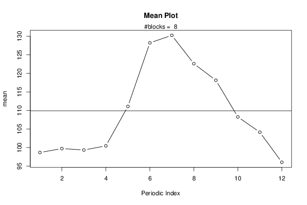
| Title produced by software | Mean Plot | ||||||||||||||||||||
| Date of computation | Fri, 11 Dec 2015 15:08:24 +0000 | ||||||||||||||||||||
| Cite this page as follows | Statistical Computations at FreeStatistics.org, Office for Research Development and Education, URL https://freestatistics.org/blog/index.php?v=date/2015/Dec/11/t1449846510qs846xutfnxvmbs.htm/, Retrieved Thu, 16 May 2024 12:02:16 +0000 | ||||||||||||||||||||
| Statistical Computations at FreeStatistics.org, Office for Research Development and Education, URL https://freestatistics.org/blog/index.php?pk=285981, Retrieved Thu, 16 May 2024 12:02:16 +0000 | |||||||||||||||||||||
| QR Codes: | |||||||||||||||||||||
|
| |||||||||||||||||||||
| Original text written by user: | |||||||||||||||||||||
| IsPrivate? | No (this computation is public) | ||||||||||||||||||||
| User-defined keywords | |||||||||||||||||||||
| Estimated Impact | 68 | ||||||||||||||||||||
Tree of Dependent Computations | |||||||||||||||||||||
| Family? (F = Feedback message, R = changed R code, M = changed R Module, P = changed Parameters, D = changed Data) | |||||||||||||||||||||
| - [Decomposition by Loess] [HPC Retail Sales] [2008-03-06 11:35:25] [74be16979710d4c4e7c6647856088456] - RMPD [Mean Plot] [] [2015-12-11 15:08:24] [09da0ac04f7f2be6cb42b66305b85db6] [Current] | |||||||||||||||||||||
| Feedback Forum | |||||||||||||||||||||
Post a new message | |||||||||||||||||||||
Dataset | |||||||||||||||||||||
| Dataseries X: | |||||||||||||||||||||
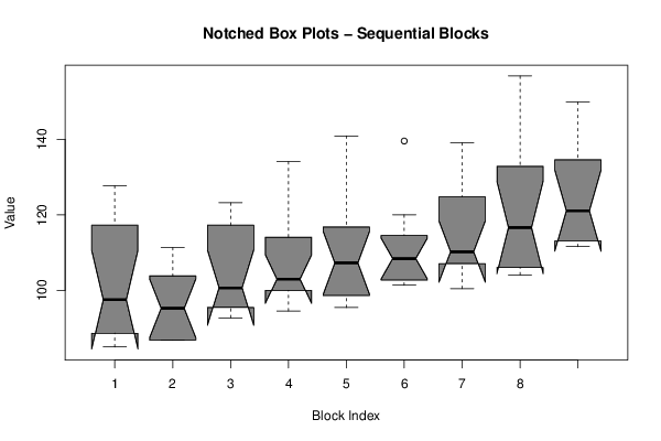
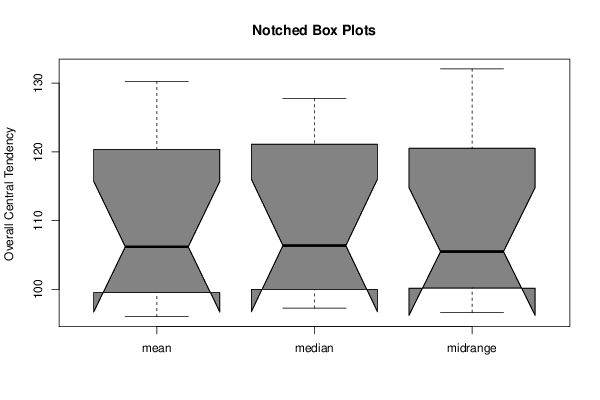
87.29 88.19 89.1 89.1 103.65 127.75 125.47 125.47 109.11 100.01 95.01 85.01 86.83 86.83 86.83 86.83 100.47 111.38 105.47 102.74 105.01 96.38 94.1 86.83 92.74 93.2 95.47 96.38 99.56 120.47 123.2 114.11 120.93 102.74 101.83 95.47 100.01 100.01 98.2 100.01 103.65 114.56 134.11 131.84 113.65 107.29 102.29 94.56 97.29 98.2 95.47 100.47 116.38 117.29 140.93 120.02 111.38 108.65 105.92 99.1 101.83 102.74 102.74 105.47 108.65 139.57 110.47 118.65 120.02 109.11 108.2 101.38 106.38 108.65 107.74 105.92 129.56 139.11 125.93 123.65 118.65 110.47 110.02 100.47 104.1 106.6 105.5 107.5 117.9 136.3 156.8 135.8 130 117.5 115.8 105.5 111.6 113.2 113.1 112.5 120 147.6 149.9 131.2 134.6 122.2 | |||||||||||||||||||||
Tables (Output of Computation) | |||||||||||||||||||||
| |||||||||||||||||||||
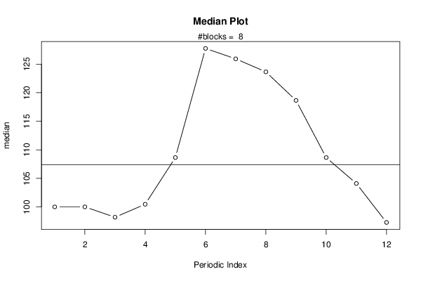
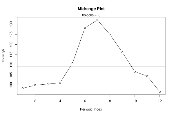
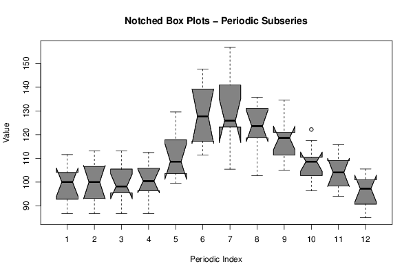
Figures (Output of Computation) | |||||||||||||||||||||
Input Parameters & R Code | |||||||||||||||||||||
| Parameters (Session): | |||||||||||||||||||||
| par1 = 12 ; | |||||||||||||||||||||
| Parameters (R input): | |||||||||||||||||||||
| par1 = 12 ; | |||||||||||||||||||||
| R code (references can be found in the software module): | |||||||||||||||||||||
par1 <- as.numeric(par1) | |||||||||||||||||||||