Free Statistics
of Irreproducible Research!
Description of Statistical Computation | |||||||||||||||||||||||||||||||||||||||
|---|---|---|---|---|---|---|---|---|---|---|---|---|---|---|---|---|---|---|---|---|---|---|---|---|---|---|---|---|---|---|---|---|---|---|---|---|---|---|---|
| Author's title | |||||||||||||||||||||||||||||||||||||||
| Author | *The author of this computation has been verified* | ||||||||||||||||||||||||||||||||||||||
| R Software Module | rwasp_fitdistrnorm.wasp | ||||||||||||||||||||||||||||||||||||||
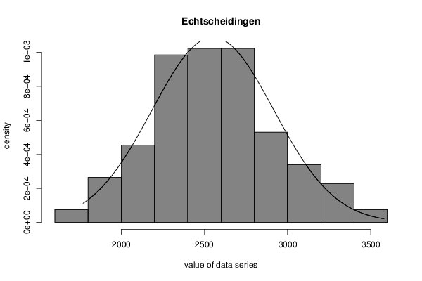
| Title produced by software | ML Fitting and QQ Plot- Normal Distribution | ||||||||||||||||||||||||||||||||||||||
| Date of computation | Fri, 11 Dec 2015 20:33:34 +0000 | ||||||||||||||||||||||||||||||||||||||
| Cite this page as follows | Statistical Computations at FreeStatistics.org, Office for Research Development and Education, URL https://freestatistics.org/blog/index.php?v=date/2015/Dec/11/t1449866022g3ttua5kqrogyu5.htm/, Retrieved Thu, 16 May 2024 04:34:33 +0000 | ||||||||||||||||||||||||||||||||||||||
| Statistical Computations at FreeStatistics.org, Office for Research Development and Education, URL https://freestatistics.org/blog/index.php?pk=286030, Retrieved Thu, 16 May 2024 04:34:33 +0000 | |||||||||||||||||||||||||||||||||||||||
| QR Codes: | |||||||||||||||||||||||||||||||||||||||
|
| |||||||||||||||||||||||||||||||||||||||
| Original text written by user: | |||||||||||||||||||||||||||||||||||||||
| IsPrivate? | No (this computation is public) | ||||||||||||||||||||||||||||||||||||||
| User-defined keywords | |||||||||||||||||||||||||||||||||||||||
| Estimated Impact | 69 | ||||||||||||||||||||||||||||||||||||||
Tree of Dependent Computations | |||||||||||||||||||||||||||||||||||||||
| Family? (F = Feedback message, R = changed R code, M = changed R Module, P = changed Parameters, D = changed Data) | |||||||||||||||||||||||||||||||||||||||
| - [ML Fitting and QQ Plot- Normal Distribution] [] [2015-12-11 20:33:34] [5fd2fca6b664199b2dd86155c5786748] [Current] | |||||||||||||||||||||||||||||||||||||||
| Feedback Forum | |||||||||||||||||||||||||||||||||||||||
Post a new message | |||||||||||||||||||||||||||||||||||||||
Dataset | |||||||||||||||||||||||||||||||||||||||
| Dataseries X: | |||||||||||||||||||||||||||||||||||||||
2132 1964 2209 1965 2631 2583 2714 2248 2364 3042 2316 2735 2493 2136 2467 2414 2556 2768 2998 2573 3005 3469 2540 3187 2689 2154 3065 2397 2787 3579 2915 3025 3245 3328 2840 3342 2261 2590 2624 1860 2577 2646 2639 2807 2350 3053 2203 2471 1967 2473 2397 1904 2732 2297 2734 2719 2296 3243 2166 2261 2408 2536 2324 2178 2803 2604 2782 2656 2801 3122 2393 2233 2451 2596 2467 2210 2948 2507 3019 2401 2818 3305 2101 2582 2407 2416 2463 2228 2616 2934 2668 2808 2664 3112 2321 2718 2297 2534 2647 2064 2642 2702 2348 2734 2709 3206 2214 2531 2119 2369 2682 1840 2622 2570 2447 2871 2485 2957 2102 2250 2051 2260 2327 1781 2631 2180 2150 2837 1976 2836 2203 1770 | |||||||||||||||||||||||||||||||||||||||
Tables (Output of Computation) | |||||||||||||||||||||||||||||||||||||||
| |||||||||||||||||||||||||||||||||||||||
Figures (Output of Computation) | |||||||||||||||||||||||||||||||||||||||
Input Parameters & R Code | |||||||||||||||||||||||||||||||||||||||
| Parameters (Session): | |||||||||||||||||||||||||||||||||||||||
| par1 = 8 ; par2 = 0 ; | |||||||||||||||||||||||||||||||||||||||
| Parameters (R input): | |||||||||||||||||||||||||||||||||||||||
| par1 = 8 ; par2 = 0 ; | |||||||||||||||||||||||||||||||||||||||
| R code (references can be found in the software module): | |||||||||||||||||||||||||||||||||||||||
library(MASS) | |||||||||||||||||||||||||||||||||||||||