Repository of Reproducible Computations

Free Statistics

of Irreproducible Research!

Author's title

Author

*The author of this computation has been verified*

R Software Module

rwasp_autocorrelation.wasp

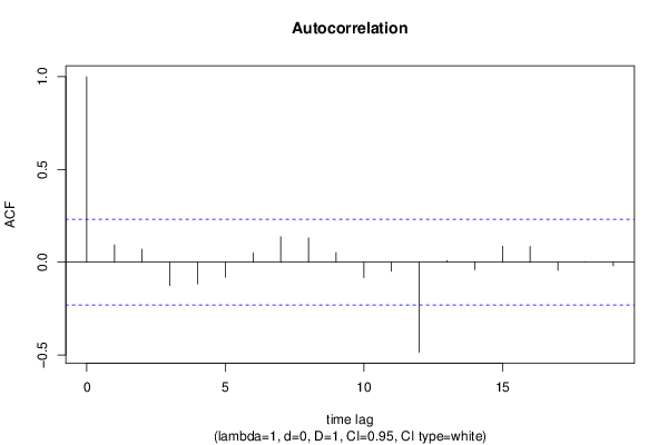
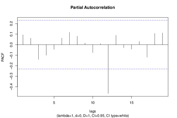
Title produced by software

(Partial) Autocorrelation Function

Date of computation

Fri, 11 Dec 2015 21:47:51 +0000

Cite this page as follows

Statistical Computations at FreeStatistics.org, Office for Research Development and Education, URL https://freestatistics.org/blog/index.php?v=date/2015/Dec/11/t1449870485d6jywivpkkxq34m.htm/, Retrieved Thu, 16 May 2024 21:25:29 +0000

Statistical Computations at FreeStatistics.org, Office for Research Development and Education, URL https://freestatistics.org/blog/index.php?pk=286038, Retrieved Thu, 16 May 2024 21:25:29 +0000

QR Codes:

Paste this QR Code to cite your computation.

Original text written by user:

IsPrivate?

No (this computation is public)

User-defined keywords

Estimated Impact

Family? (F = Feedback message, R = changed R code, M = changed R Module, P = changed Parameters, D = changed Data)

-     [Two-Way ANOVA] [] [2015-11-16 17:14:42] [32b17a345b130fdf5cc88718ed94a974]
- RMPD  [Exponential Smoothing] [] [2015-12-11 21:11:55] [0e2e3dbefef1c665f3752d42409bac25]
- RM D      [(Partial) Autocorrelation Function] [] [2015-12-11 21:47:51] [074449c5cdcdb4dafd7dd3585d12ae02] [Current]
- RM D        [Box-Cox Linearity Plot] [] [2015-12-11 21:55:28] [0e2e3dbefef1c665f3752d42409bac25] 
- RM D        [Box-Cox Normality Plot] [] [2015-12-11 21:57:36] [0e2e3dbefef1c665f3752d42409bac25] 
- R           [(Partial) Autocorrelation Function] [] [2015-12-11 22:01:00] [0e2e3dbefef1c665f3752d42409bac25] 
- RM D        [ARIMA Backward Selection] [] [2015-12-11 22:02:14] [0e2e3dbefef1c665f3752d42409bac25] 
- RM D        [Kendall tau Correlation Matrix] [] [2015-12-11 22:11:18] [0e2e3dbefef1c665f3752d42409bac25] 

Feedback Forum

Post a new message

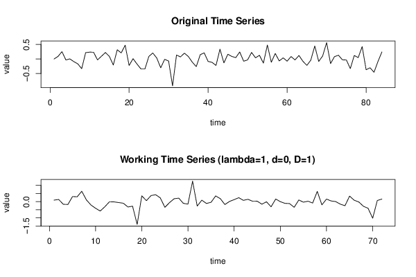
Dataseries X:

Download CSV

Histogram

Boxplots

0.0013999990894105
0.0876771622176185
0.253920154859331
-0.0329407507841036
0.00427395855379008
-0.0889668134958849
-0.165281368150775
-0.33220433089751
0.219927126513421
0.236701919529402
0.234525437835356
-0.0304289243382355
0.0953913592916723
0.222671044416315
0.0914666084830592
-0.206034580848975
0.317983507811223
0.209887369047125
0.47505736015715
-0.222062521324981
0.0119408639911758
-0.172481528037084
-0.342720660187122
-0.343867756086308
0.088435724392957
0.207149951929822
0.0343760117343465
-0.301707672057424
-0.0110173444677831
-0.0691482212286872
-0.925838573157798
0.137673245546374
0.0727565374056945
0.201173883123843
0.0856783035058499
-0.109577212438584
-0.260551934204086
0.147885882041203
0.212413648519748
-0.0832851309957541
-0.115216896092894
-0.221533847078893
0.33793754507397
-0.134446101735477
0.164631582429395
0.0888222485881065
0.0469533479921545
0.241738416214495
-0.0752540261587926
-0.0299598595890917
0.225881103587503
0.0412636104361186
0.128108276344458
-0.141250457347375
0.481091241511557
-0.11016711751824
0.191801843198123
-0.066757083135655
0.0394798962983962
-0.0743907512944395
0.0864476825544102
-0.0321810065262648
0.121406171476103
-0.0784677853924106
-0.219288911182277
-0.0373619502368736
0.449190378168538
-0.083495394142657
0.104571843583723
0.564217976443139
-0.156913984252991
0.0837627464269975
0.129666943943497
-0.0279018187223396
-0.0344326851573588
-0.328655799589801
0.121385421475263
0.0494710079304724
0.428353319793773
-0.368885964978714
-0.302589451991359
-0.45541145100303
-0.0851366312257987
0.244537840690697

Summary of computational transaction
Raw Input	view raw input (R code)
Raw Output	view raw output of R engine
Computing time	2 seconds
R Server	'Sir Maurice George Kendall' @ kendall.wessa.net

\begin{tabular}{lllllllll}
\hline
Summary of computational transaction \tabularnewline
Raw Input & view raw input (R code)  \tabularnewline
Raw Output & view raw output of R engine  \tabularnewline
Computing time & 2 seconds \tabularnewline
R Server & 'Sir Maurice George Kendall' @ kendall.wessa.net \tabularnewline
\hline
\end{tabular}
%Source: https://freestatistics.org/blog/index.php?pk=286038&T=0

[TABLE]
[ROW][C]Summary of computational transaction[/C][/ROW]
[ROW][C]Raw Input[/C][C]view raw input (R code) [/C][/ROW]
[ROW][C]Raw Output[/C][C]view raw output of R engine [/C][/ROW]
[ROW][C]Computing time[/C][C]2 seconds[/C][/ROW]
[ROW][C]R Server[/C][C]'Sir Maurice George Kendall' @ kendall.wessa.net[/C][/ROW]
[/TABLE]
Source: https://freestatistics.org/blog/index.php?pk=286038&T=0

Globally Unique Identifier (entire table): ba.freestatistics.org/blog/index.php?pk=286038&T=0

As an alternative you can also use a QR Code:

The GUIDs for individual cells are displayed in the table below:

Summary of computational transaction
Raw Input	view raw input (R code)
Raw Output	view raw output of R engine
Computing time	2 seconds
R Server	'Sir Maurice George Kendall' @ kendall.wessa.net

Autocorrelation Function
Time lag k	ACF(k)	T-STAT	P-value
1	0.093177	0.7906	0.215876
2	0.06976	0.5919	0.277875
3	-0.125829	-1.0677	0.144613
4	-0.117388	-0.9961	0.161275
5	-0.081384	-0.6906	0.246029
6	0.049685	0.4216	0.337291
7	0.137899	1.1701	0.122908
8	0.130628	1.1084	0.135686
9	0.051241	0.4348	0.332505
10	-0.083287	-0.7067	0.241012
11	-0.04917	-0.4172	0.338881
12	-0.485895	-4.123	4.9e-05
13	0.008245	0.07	0.47221
14	-0.041512	-0.3522	0.362844
15	0.086458	0.7336	0.232782
16	0.084856	0.72	0.236919
17	-0.044029	-0.3736	0.3549
18	-7e-04	-0.0059	0.497637
19	-0.019666	-0.1669	0.433968

\begin{tabular}{lllllllll}
\hline
Autocorrelation Function \tabularnewline
Time lag k & ACF(k) & T-STAT & P-value \tabularnewline
1 & 0.093177 & 0.7906 & 0.215876 \tabularnewline
2 & 0.06976 & 0.5919 & 0.277875 \tabularnewline
3 & -0.125829 & -1.0677 & 0.144613 \tabularnewline
4 & -0.117388 & -0.9961 & 0.161275 \tabularnewline
5 & -0.081384 & -0.6906 & 0.246029 \tabularnewline
6 & 0.049685 & 0.4216 & 0.337291 \tabularnewline
7 & 0.137899 & 1.1701 & 0.122908 \tabularnewline
8 & 0.130628 & 1.1084 & 0.135686 \tabularnewline
9 & 0.051241 & 0.4348 & 0.332505 \tabularnewline
10 & -0.083287 & -0.7067 & 0.241012 \tabularnewline
11 & -0.04917 & -0.4172 & 0.338881 \tabularnewline
12 & -0.485895 & -4.123 & 4.9e-05 \tabularnewline
13 & 0.008245 & 0.07 & 0.47221 \tabularnewline
14 & -0.041512 & -0.3522 & 0.362844 \tabularnewline
15 & 0.086458 & 0.7336 & 0.232782 \tabularnewline
16 & 0.084856 & 0.72 & 0.236919 \tabularnewline
17 & -0.044029 & -0.3736 & 0.3549 \tabularnewline
18 & -7e-04 & -0.0059 & 0.497637 \tabularnewline
19 & -0.019666 & -0.1669 & 0.433968 \tabularnewline
\hline
\end{tabular}
%Source: https://freestatistics.org/blog/index.php?pk=286038&T=1

[TABLE]
[ROW][C]Autocorrelation Function[/C][/ROW]
[ROW][C]Time lag k[/C][C]ACF(k)[/C][C]T-STAT[/C][C]P-value[/C][/ROW]
[ROW][C]1[/C][C]0.093177[/C][C]0.7906[/C][C]0.215876[/C][/ROW]
[ROW][C]2[/C][C]0.06976[/C][C]0.5919[/C][C]0.277875[/C][/ROW]
[ROW][C]3[/C][C]-0.125829[/C][C]-1.0677[/C][C]0.144613[/C][/ROW]
[ROW][C]4[/C][C]-0.117388[/C][C]-0.9961[/C][C]0.161275[/C][/ROW]
[ROW][C]5[/C][C]-0.081384[/C][C]-0.6906[/C][C]0.246029[/C][/ROW]
[ROW][C]6[/C][C]0.049685[/C][C]0.4216[/C][C]0.337291[/C][/ROW]
[ROW][C]7[/C][C]0.137899[/C][C]1.1701[/C][C]0.122908[/C][/ROW]
[ROW][C]8[/C][C]0.130628[/C][C]1.1084[/C][C]0.135686[/C][/ROW]
[ROW][C]9[/C][C]0.051241[/C][C]0.4348[/C][C]0.332505[/C][/ROW]
[ROW][C]10[/C][C]-0.083287[/C][C]-0.7067[/C][C]0.241012[/C][/ROW]
[ROW][C]11[/C][C]-0.04917[/C][C]-0.4172[/C][C]0.338881[/C][/ROW]
[ROW][C]12[/C][C]-0.485895[/C][C]-4.123[/C][C]4.9e-05[/C][/ROW]
[ROW][C]13[/C][C]0.008245[/C][C]0.07[/C][C]0.47221[/C][/ROW]
[ROW][C]14[/C][C]-0.041512[/C][C]-0.3522[/C][C]0.362844[/C][/ROW]
[ROW][C]15[/C][C]0.086458[/C][C]0.7336[/C][C]0.232782[/C][/ROW]
[ROW][C]16[/C][C]0.084856[/C][C]0.72[/C][C]0.236919[/C][/ROW]
[ROW][C]17[/C][C]-0.044029[/C][C]-0.3736[/C][C]0.3549[/C][/ROW]
[ROW][C]18[/C][C]-7e-04[/C][C]-0.0059[/C][C]0.497637[/C][/ROW]
[ROW][C]19[/C][C]-0.019666[/C][C]-0.1669[/C][C]0.433968[/C][/ROW]
[/TABLE]
Source: https://freestatistics.org/blog/index.php?pk=286038&T=1

Globally Unique Identifier (entire table): ba.freestatistics.org/blog/index.php?pk=286038&T=1

As an alternative you can also use a QR Code:

The GUIDs for individual cells are displayed in the table below:

Autocorrelation Function
Time lag k	ACF(k)	T-STAT	P-value
1	0.093177	0.7906	0.215876
2	0.06976	0.5919	0.277875
3	-0.125829	-1.0677	0.144613
4	-0.117388	-0.9961	0.161275
5	-0.081384	-0.6906	0.246029
6	0.049685	0.4216	0.337291
7	0.137899	1.1701	0.122908
8	0.130628	1.1084	0.135686
9	0.051241	0.4348	0.332505
10	-0.083287	-0.7067	0.241012
11	-0.04917	-0.4172	0.338881
12	-0.485895	-4.123	4.9e-05
13	0.008245	0.07	0.47221
14	-0.041512	-0.3522	0.362844
15	0.086458	0.7336	0.232782
16	0.084856	0.72	0.236919
17	-0.044029	-0.3736	0.3549
18	-7e-04	-0.0059	0.497637
19	-0.019666	-0.1669	0.433968

Partial Autocorrelation Function
Time lag k	PACF(k)	T-STAT	P-value
1	0.093177	0.7906	0.215876
2	0.061613	0.5228	0.301359
3	-0.139404	-1.1829	0.120374
4	-0.100649	-0.854	0.19796
5	-0.044973	-0.3816	0.351937
6	0.062647	0.5316	0.298328
7	0.117027	0.993	0.162017
8	0.079993	0.6788	0.249731
9	0.015626	0.1326	0.447443
10	-0.075605	-0.6415	0.261609
11	0.009528	0.0808	0.467894
12	-0.463129	-3.9298	9.7e-05
13	0.088386	0.75	0.227855
14	-0.02943	-0.2497	0.401756
15	-0.043462	-0.3688	0.356685
16	0.03097	0.2628	0.396731
17	-0.118484	-1.0054	0.159043
18	0.106861	0.9067	0.183782
19	0.111318	0.9446	0.174019

\begin{tabular}{lllllllll}
\hline
Partial Autocorrelation Function \tabularnewline
Time lag k & PACF(k) & T-STAT & P-value \tabularnewline
1 & 0.093177 & 0.7906 & 0.215876 \tabularnewline
2 & 0.061613 & 0.5228 & 0.301359 \tabularnewline
3 & -0.139404 & -1.1829 & 0.120374 \tabularnewline
4 & -0.100649 & -0.854 & 0.19796 \tabularnewline
5 & -0.044973 & -0.3816 & 0.351937 \tabularnewline
6 & 0.062647 & 0.5316 & 0.298328 \tabularnewline
7 & 0.117027 & 0.993 & 0.162017 \tabularnewline
8 & 0.079993 & 0.6788 & 0.249731 \tabularnewline
9 & 0.015626 & 0.1326 & 0.447443 \tabularnewline
10 & -0.075605 & -0.6415 & 0.261609 \tabularnewline
11 & 0.009528 & 0.0808 & 0.467894 \tabularnewline
12 & -0.463129 & -3.9298 & 9.7e-05 \tabularnewline
13 & 0.088386 & 0.75 & 0.227855 \tabularnewline
14 & -0.02943 & -0.2497 & 0.401756 \tabularnewline
15 & -0.043462 & -0.3688 & 0.356685 \tabularnewline
16 & 0.03097 & 0.2628 & 0.396731 \tabularnewline
17 & -0.118484 & -1.0054 & 0.159043 \tabularnewline
18 & 0.106861 & 0.9067 & 0.183782 \tabularnewline
19 & 0.111318 & 0.9446 & 0.174019 \tabularnewline
\hline
\end{tabular}
%Source: https://freestatistics.org/blog/index.php?pk=286038&T=2

[TABLE]
[ROW][C]Partial Autocorrelation Function[/C][/ROW]
[ROW][C]Time lag k[/C][C]PACF(k)[/C][C]T-STAT[/C][C]P-value[/C][/ROW]
[ROW][C]1[/C][C]0.093177[/C][C]0.7906[/C][C]0.215876[/C][/ROW]
[ROW][C]2[/C][C]0.061613[/C][C]0.5228[/C][C]0.301359[/C][/ROW]
[ROW][C]3[/C][C]-0.139404[/C][C]-1.1829[/C][C]0.120374[/C][/ROW]
[ROW][C]4[/C][C]-0.100649[/C][C]-0.854[/C][C]0.19796[/C][/ROW]
[ROW][C]5[/C][C]-0.044973[/C][C]-0.3816[/C][C]0.351937[/C][/ROW]
[ROW][C]6[/C][C]0.062647[/C][C]0.5316[/C][C]0.298328[/C][/ROW]
[ROW][C]7[/C][C]0.117027[/C][C]0.993[/C][C]0.162017[/C][/ROW]
[ROW][C]8[/C][C]0.079993[/C][C]0.6788[/C][C]0.249731[/C][/ROW]
[ROW][C]9[/C][C]0.015626[/C][C]0.1326[/C][C]0.447443[/C][/ROW]
[ROW][C]10[/C][C]-0.075605[/C][C]-0.6415[/C][C]0.261609[/C][/ROW]
[ROW][C]11[/C][C]0.009528[/C][C]0.0808[/C][C]0.467894[/C][/ROW]
[ROW][C]12[/C][C]-0.463129[/C][C]-3.9298[/C][C]9.7e-05[/C][/ROW]
[ROW][C]13[/C][C]0.088386[/C][C]0.75[/C][C]0.227855[/C][/ROW]
[ROW][C]14[/C][C]-0.02943[/C][C]-0.2497[/C][C]0.401756[/C][/ROW]
[ROW][C]15[/C][C]-0.043462[/C][C]-0.3688[/C][C]0.356685[/C][/ROW]
[ROW][C]16[/C][C]0.03097[/C][C]0.2628[/C][C]0.396731[/C][/ROW]
[ROW][C]17[/C][C]-0.118484[/C][C]-1.0054[/C][C]0.159043[/C][/ROW]
[ROW][C]18[/C][C]0.106861[/C][C]0.9067[/C][C]0.183782[/C][/ROW]
[ROW][C]19[/C][C]0.111318[/C][C]0.9446[/C][C]0.174019[/C][/ROW]
[/TABLE]
Source: https://freestatistics.org/blog/index.php?pk=286038&T=2

Globally Unique Identifier (entire table): ba.freestatistics.org/blog/index.php?pk=286038&T=2

As an alternative you can also use a QR Code:

The GUIDs for individual cells are displayed in the table below:

Partial Autocorrelation Function
Time lag k	PACF(k)	T-STAT	P-value
1	0.093177	0.7906	0.215876
2	0.061613	0.5228	0.301359
3	-0.139404	-1.1829	0.120374
4	-0.100649	-0.854	0.19796
5	-0.044973	-0.3816	0.351937
6	0.062647	0.5316	0.298328
7	0.117027	0.993	0.162017
8	0.079993	0.6788	0.249731
9	0.015626	0.1326	0.447443
10	-0.075605	-0.6415	0.261609
11	0.009528	0.0808	0.467894
12	-0.463129	-3.9298	9.7e-05
13	0.088386	0.75	0.227855
14	-0.02943	-0.2497	0.401756
15	-0.043462	-0.3688	0.356685
16	0.03097	0.2628	0.396731
17	-0.118484	-1.0054	0.159043
18	0.106861	0.9067	0.183782
19	0.111318	0.9446	0.174019

Figure 1

PNG link

Postscript link

PDF link

Figure 2

PNG link

Postscript link

PDF link

Figure 3

PNG link

Postscript link

PDF link

Parameters (Session):

Parameters (R input):

par1 = Default ; par2 = 1 ; par3 = 0 ; par4 = 1 ; par5 = 12 ; par6 = White Noise ; par7 = 0.95 ; par8 = ;

R code (references can be found in the software module):

par8 <- ''
par7 <- '0.95'
par6 <- 'White Noise'
par5 <- '12'
par4 <- '0'
par3 <- '1'
par2 <- '1'
par1 <- 'Default'
if (par1 == 'Default') {
par1 = 10*log10(length(x))
} else {
par1 <- as.numeric(par1)
}
par2 <- as.numeric(par2)
par3 <- as.numeric(par3)
par4 <- as.numeric(par4)
par5 <- as.numeric(par5)
if (par6 == 'White Noise') par6 <- 'white' else par6 <- 'ma'
par7 <- as.numeric(par7)
if (par8 != '') par8 <- as.numeric(par8)
x <- na.omit(x)
ox <- x
if (par8 == '') {
if (par2 == 0) {
x <- log(x)
} else {
x <- (x ^ par2 - 1) / par2
}
} else {
x <- log(x,base=par8)
}
if (par3 > 0) x <- diff(x,lag=1,difference=par3)
if (par4 > 0) x <- diff(x,lag=par5,difference=par4)
bitmap(file='picts.png')
op <- par(mfrow=c(2,1))
plot(ox,type='l',main='Original Time Series',xlab='time',ylab='value')
if (par8=='') {
mytitle <- paste('Working Time Series (lambda=',par2,', d=',par3,', D=',par4,')',sep='')
mysub <- paste('(lambda=',par2,', d=',par3,', D=',par4,', CI=', par7, ', CI type=',par6,')',sep='')
} else {
mytitle <- paste('Working Time Series (base=',par8,', d=',par3,', D=',par4,')',sep='')
mysub <- paste('(base=',par8,', d=',par3,', D=',par4,', CI=', par7, ', CI type=',par6,')',sep='')
}
plot(x,type='l', main=mytitle,xlab='time',ylab='value')
par(op)
dev.off()
bitmap(file='pic1.png')
racf <- acf(x, par1, main='Autocorrelation', xlab='time lag', ylab='ACF', ci.type=par6, ci=par7, sub=mysub)
dev.off()
bitmap(file='pic2.png')
rpacf <- pacf(x,par1,main='Partial Autocorrelation',xlab='lags',ylab='PACF',sub=mysub)
dev.off()
(myacf <- c(racf$acf))
(mypacf <- c(rpacf$acf))
lengthx <- length(x)
sqrtn <- sqrt(lengthx)
load(file='createtable')
a<-table.start()
a<-table.row.start(a)
a<-table.element(a,'Autocorrelation Function',4,TRUE)
a<-table.row.end(a)
a<-table.row.start(a)
a<-table.element(a,'Time lag k',header=TRUE)
a<-table.element(a,hyperlink('basics.htm','ACF(k)','click here for more information about the Autocorrelation Function'),header=TRUE)
a<-table.element(a,'T-STAT',header=TRUE)
a<-table.element(a,'P-value',header=TRUE)
a<-table.row.end(a)
for (i in 2:(par1+1)) {
a<-table.row.start(a)
a<-table.element(a,i-1,header=TRUE)
a<-table.element(a,round(myacf[i],6))
mytstat <- myacf[i]*sqrtn
a<-table.element(a,round(mytstat,4))
a<-table.element(a,round(1-pt(abs(mytstat),lengthx),6))
a<-table.row.end(a)
}
a<-table.end(a)
table.save(a,file='mytable.tab')
a<-table.start()
a<-table.row.start(a)
a<-table.element(a,'Partial Autocorrelation Function',4,TRUE)
a<-table.row.end(a)
a<-table.row.start(a)
a<-table.element(a,'Time lag k',header=TRUE)
a<-table.element(a,hyperlink('basics.htm','PACF(k)','click here for more information about the Partial Autocorrelation Function'),header=TRUE)
a<-table.element(a,'T-STAT',header=TRUE)
a<-table.element(a,'P-value',header=TRUE)
a<-table.row.end(a)
for (i in 1:par1) {
a<-table.row.start(a)
a<-table.element(a,i,header=TRUE)
a<-table.element(a,round(mypacf[i],6))
mytstat <- mypacf[i]*sqrtn
a<-table.element(a,round(mytstat,4))
a<-table.element(a,round(1-pt(abs(mytstat),lengthx),6))
a<-table.row.end(a)
}
a<-table.end(a)
table.save(a,file='mytable1.tab')

Free Statistics

Description of Statistical Computation

Tree of Dependent Computations

Dataset

Tables (Output of Computation)

Figures (Output of Computation)

Input Parameters & R Code