Free Statistics
of Irreproducible Research!
Description of Statistical Computation | |||||||||||||||||||||||||||||||||||||||||
|---|---|---|---|---|---|---|---|---|---|---|---|---|---|---|---|---|---|---|---|---|---|---|---|---|---|---|---|---|---|---|---|---|---|---|---|---|---|---|---|---|---|
| Author's title | |||||||||||||||||||||||||||||||||||||||||
| Author | *The author of this computation has been verified* | ||||||||||||||||||||||||||||||||||||||||
| R Software Module | rwasp_univariatedataseries.wasp | ||||||||||||||||||||||||||||||||||||||||
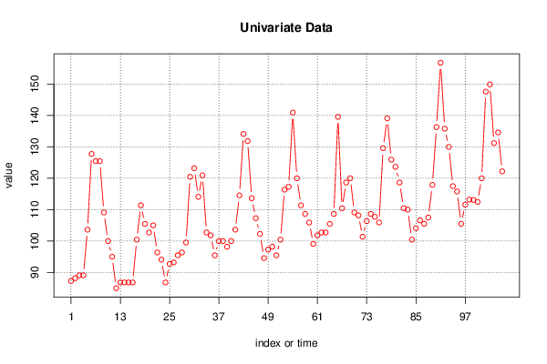
| Title produced by software | Univariate Data Series | ||||||||||||||||||||||||||||||||||||||||
| Date of computation | Wed, 16 Dec 2015 19:09:29 +0000 | ||||||||||||||||||||||||||||||||||||||||
| Cite this page as follows | Statistical Computations at FreeStatistics.org, Office for Research Development and Education, URL https://freestatistics.org/blog/index.php?v=date/2015/Dec/16/t14502929835y1qowkhya5u9j4.htm/, Retrieved Thu, 16 May 2024 20:54:43 +0000 | ||||||||||||||||||||||||||||||||||||||||
| Statistical Computations at FreeStatistics.org, Office for Research Development and Education, URL https://freestatistics.org/blog/index.php?pk=286736, Retrieved Thu, 16 May 2024 20:54:43 +0000 | |||||||||||||||||||||||||||||||||||||||||
| QR Codes: | |||||||||||||||||||||||||||||||||||||||||
|
| |||||||||||||||||||||||||||||||||||||||||
| Original text written by user: | |||||||||||||||||||||||||||||||||||||||||
| IsPrivate? | No (this computation is public) | ||||||||||||||||||||||||||||||||||||||||
| User-defined keywords | |||||||||||||||||||||||||||||||||||||||||
| Estimated Impact | 80 | ||||||||||||||||||||||||||||||||||||||||
Tree of Dependent Computations | |||||||||||||||||||||||||||||||||||||||||
| Family? (F = Feedback message, R = changed R code, M = changed R Module, P = changed Parameters, D = changed Data) | |||||||||||||||||||||||||||||||||||||||||
| - [Univariate Data Series] [] [2015-12-16 19:09:29] [0f06e4fdd8087d4b3abca42184bf2a00] [Current] - RMP [Mean Plot] [] [2015-12-16 19:15:48] [c4d175d45982400f45768592120a8602] - RM [Variance Reduction Matrix] [] [2015-12-16 19:29:45] [c4d175d45982400f45768592120a8602] - RMP [(Partial) Autocorrelation Function] [] [2015-12-16 19:34:59] [c4d175d45982400f45768592120a8602] - RMP [(Partial) Autocorrelation Function] [] [2015-12-16 19:37:59] [c4d175d45982400f45768592120a8602] | |||||||||||||||||||||||||||||||||||||||||
| Feedback Forum | |||||||||||||||||||||||||||||||||||||||||
Post a new message | |||||||||||||||||||||||||||||||||||||||||
Dataset | |||||||||||||||||||||||||||||||||||||||||
| Dataseries X: | |||||||||||||||||||||||||||||||||||||||||
87.29 88.19 89.1 89.1 103.65 127.75 125.47 125.47 109.11 100.01 95.01 85.01 86.83 86.83 86.83 86.83 100.47 111.38 105.47 102.74 105.01 96.38 94.1 86.83 92.74 93.2 95.47 96.38 99.56 120.47 123.2 114.11 120.93 102.74 101.83 95.47 100.01 100.01 98.2 100.01 103.65 114.56 134.11 131.84 113.65 107.29 102.29 94.56 97.29 98.2 95.47 100.47 116.38 117.29 140.93 120.02 111.38 108.65 105.92 99.1 101.83 102.74 102.74 105.47 108.65 139.57 110.47 118.65 120.02 109.11 108.2 101.38 106.38 108.65 107.74 105.92 129.56 139.11 125.93 123.65 118.65 110.47 110.02 100.47 104.1 106.6 105.5 107.5 117.9 136.3 156.8 135.8 130 117.5 115.8 105.5 111.6 113.2 113.1 112.5 120 147.6 149.9 131.2 134.6 122.2 | |||||||||||||||||||||||||||||||||||||||||
Tables (Output of Computation) | |||||||||||||||||||||||||||||||||||||||||
| |||||||||||||||||||||||||||||||||||||||||
Figures (Output of Computation) | |||||||||||||||||||||||||||||||||||||||||
Input Parameters & R Code | |||||||||||||||||||||||||||||||||||||||||
| Parameters (Session): | |||||||||||||||||||||||||||||||||||||||||
| par1 = Gemiddeld waterverbruik in London, Ontario ; par2 = https://datamarket.com/data/set/22qu/monthly-water-usage-mlday-london-ontario-1966-1988#!ds=22qu&display=line ; par3 = Maandelijks waterverbruik in London, Ontario, uitgedrukt in Ml/dag voor de periode januari 1971- oktober 1979 ; par4 = 12 ; | |||||||||||||||||||||||||||||||||||||||||
| Parameters (R input): | |||||||||||||||||||||||||||||||||||||||||
| par1 = Gemiddeld waterverbruik in London, Ontario ; par2 = https://datamarket.com/data/set/22qu/monthly-water-usage-mlday-london-ontario-1966-1988#!ds=22qu&display=line ; par3 = Maandelijks waterverbruik in London, Ontario, uitgedrukt in Ml/dag voor de periode januari 1971- oktober 1979 ; par4 = 12 ; | |||||||||||||||||||||||||||||||||||||||||
| R code (references can be found in the software module): | |||||||||||||||||||||||||||||||||||||||||
par4 <- '12' | |||||||||||||||||||||||||||||||||||||||||