Free Statistics
of Irreproducible Research!
Description of Statistical Computation | |||||||||||||||||||||||||||||||||||||||||||||||||
|---|---|---|---|---|---|---|---|---|---|---|---|---|---|---|---|---|---|---|---|---|---|---|---|---|---|---|---|---|---|---|---|---|---|---|---|---|---|---|---|---|---|---|---|---|---|---|---|---|---|
| Author's title | |||||||||||||||||||||||||||||||||||||||||||||||||
| Author | *The author of this computation has been verified* | ||||||||||||||||||||||||||||||||||||||||||||||||
| R Software Module | rwasp_tukeylambda.wasp | ||||||||||||||||||||||||||||||||||||||||||||||||
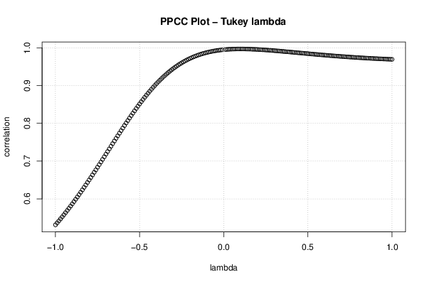
| Title produced by software | Tukey lambda PPCC Plot | ||||||||||||||||||||||||||||||||||||||||||||||||
| Date of computation | Fri, 18 Dec 2015 09:58:56 +0000 | ||||||||||||||||||||||||||||||||||||||||||||||||
| Cite this page as follows | Statistical Computations at FreeStatistics.org, Office for Research Development and Education, URL https://freestatistics.org/blog/index.php?v=date/2015/Dec/18/t1450432754tu4537dk414weha.htm/, Retrieved Thu, 16 May 2024 21:50:01 +0000 | ||||||||||||||||||||||||||||||||||||||||||||||||
| Statistical Computations at FreeStatistics.org, Office for Research Development and Education, URL https://freestatistics.org/blog/index.php?pk=286864, Retrieved Thu, 16 May 2024 21:50:01 +0000 | |||||||||||||||||||||||||||||||||||||||||||||||||
| QR Codes: | |||||||||||||||||||||||||||||||||||||||||||||||||
|
| |||||||||||||||||||||||||||||||||||||||||||||||||
| Original text written by user: | |||||||||||||||||||||||||||||||||||||||||||||||||
| IsPrivate? | No (this computation is public) | ||||||||||||||||||||||||||||||||||||||||||||||||
| User-defined keywords | |||||||||||||||||||||||||||||||||||||||||||||||||
| Estimated Impact | 109 | ||||||||||||||||||||||||||||||||||||||||||||||||
Tree of Dependent Computations | |||||||||||||||||||||||||||||||||||||||||||||||||
| Family? (F = Feedback message, R = changed R code, M = changed R Module, P = changed Parameters, D = changed Data) | |||||||||||||||||||||||||||||||||||||||||||||||||
| - [Tukey lambda PPCC Plot] [tukey lambda - head] [2015-12-11 11:39:49] [bcd8153d44f369b7624d3c1b4621c4c3] - D [Tukey lambda PPCC Plot] [] [2015-12-18 09:58:56] [a05da232bd4bc389022edd498fae0565] [Current] | |||||||||||||||||||||||||||||||||||||||||||||||||
| Feedback Forum | |||||||||||||||||||||||||||||||||||||||||||||||||
Post a new message | |||||||||||||||||||||||||||||||||||||||||||||||||
Dataset | |||||||||||||||||||||||||||||||||||||||||||||||||
| Dataseries X: | |||||||||||||||||||||||||||||||||||||||||||||||||
1530 1297 1335 1282 1590 1300 1400 1255 1355 1375 1340 1380 1355 1522 1208 1405 1358 1292 1340 1400 1357 1287 1275 1270 1635 1505 1490 1485 1310 1420 1318 1432 1364 1405 1432 1207 1375 1350 1236 1250 1350 1320 1525 1570 1340 1422 1506 1215 1311 1300 1224 1350 1335 1390 1400 1225 1310 1560 1330 1222 1415 1175 1330 1485 1470 1135 1310 1154 1510 1415 1468 1390 1380 1432 1240 1195 1225 1188 1252 1315 1245 1430 1279 1245 1309 1412 1120 1220 1280 1440 1370 1192 1230 1346 1290 1165 1240 1132 1242 1270 1218 1430 1588 1320 1290 1260 1425 1226 1360 1620 1310 1250 1295 1290 1290 1275 1250 1270 1362 1300 1173 1256 1440 1180 1306 1350 1125 1165 1312 1300 1270 1335 1450 1310 1027 1235 1260 1165 1080 1127 1270 1252 1200 1290 1334 1380 1140 1243 1340 1168 1322 1249 1321 1192 1373 1170 1265 1235 1302 1241 1078 1520 1460 1075 1280 1180 1250 1190 1374 1306 1202 1240 1316 1280 1350 1180 1210 1127 1324 1210 1290 1100 1280 1175 1160 1205 1163 1022 1243 1350 1237 1204 1090 1355 1250 1076 1120 1220 1240 1220 1095 1235 1105 1405 1150 1305 1220 1296 1175 955 1070 1320 1060 1130 1250 1225 1180 1178 1142 1130 1185 1012 1280 1103 1408 1300 1246 1380 1350 1060 1350 1220 1110 1215 1104 1170 1120 | |||||||||||||||||||||||||||||||||||||||||||||||||
Tables (Output of Computation) | |||||||||||||||||||||||||||||||||||||||||||||||||
| |||||||||||||||||||||||||||||||||||||||||||||||||
Figures (Output of Computation) | |||||||||||||||||||||||||||||||||||||||||||||||||
Input Parameters & R Code | |||||||||||||||||||||||||||||||||||||||||||||||||
| Parameters (Session): | |||||||||||||||||||||||||||||||||||||||||||||||||
| Parameters (R input): | |||||||||||||||||||||||||||||||||||||||||||||||||
| R code (references can be found in the software module): | |||||||||||||||||||||||||||||||||||||||||||||||||
gp <- function(lambda, p) | |||||||||||||||||||||||||||||||||||||||||||||||||