\begin{tabular}{lllllllll}
\hline
Summary of computational transaction \tabularnewline
Raw Input & view raw input (R code)  \tabularnewline
Raw Output & view raw output of R engine  \tabularnewline
Computing time & 1 seconds \tabularnewline
R Server & 'Sir Ronald Aylmer Fisher' @ fisher.wessa.net \tabularnewline
\hline
\end{tabular}
%Source: https://freestatistics.org/blog/index.php?pk=280947&T=0
[TABLE]
[ROW][C]Summary of computational transaction[/C][/ROW]
[ROW][C]Raw Input[/C][C]view raw input (R code) [/C][/ROW]
[ROW][C]Raw Output[/C][C]view raw output of R engine [/C][/ROW]
[ROW][C]Computing time[/C][C]1 seconds[/C][/ROW]
[ROW][C]R Server[/C][C]'Sir Ronald Aylmer Fisher' @ fisher.wessa.net[/C][/ROW]
[/TABLE]
Source: https://freestatistics.org/blog/index.php?pk=280947&T=0
If you paste this QR Code into your document, anyone with a smartphone or tablet will be able to scan it and view this table in a browser.
If you paste this QR Code into your document, anyone with a smartphone or tablet will be able to scan it and view this table in a browser.
If you paste this QR Code into your document, anyone with a smartphone or tablet will be able to scan it and view this table in a browser.
If you paste this QR Code into your document, anyone with a smartphone or tablet will be able to scan it and view this table in a browser.
If you paste this QR Code into your document, anyone with a smartphone or tablet will be able to scan it and view this table in a browser.
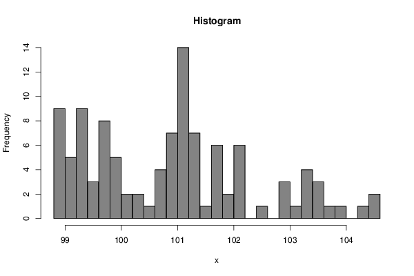
| Frequency Table (Histogram) | | Bins | Midpoint | Abs. Frequency | Rel. Frequency | Cumul. Rel. Freq. | Density | | [98.8,99[ | 98.9 | 9 | 0.083333 | 0.083333 | 0.416667 | | [99,99.2[ | 99.1 | 5 | 0.046296 | 0.12963 | 0.231481 | | [99.2,99.4[ | 99.3 | 9 | 0.083333 | 0.212963 | 0.416667 | | [99.4,99.6[ | 99.5 | 3 | 0.027778 | 0.240741 | 0.138889 | | [99.6,99.8[ | 99.7 | 8 | 0.074074 | 0.314815 | 0.37037 | | [99.8,100[ | 99.9 | 5 | 0.046296 | 0.361111 | 0.231481 | | [100,100.2[ | 100.1 | 2 | 0.018519 | 0.37963 | 0.092593 | | [100.2,100.4[ | 100.3 | 2 | 0.018519 | 0.398148 | 0.092593 | | [100.4,100.6[ | 100.5 | 1 | 0.009259 | 0.407407 | 0.046296 | | [100.6,100.8[ | 100.7 | 4 | 0.037037 | 0.444444 | 0.185185 | | [100.8,101[ | 100.9 | 7 | 0.064815 | 0.509259 | 0.324074 | | [101,101.2[ | 101.1 | 14 | 0.12963 | 0.638889 | 0.648148 | | [101.2,101.4[ | 101.3 | 7 | 0.064815 | 0.703704 | 0.324074 | | [101.4,101.6[ | 101.5 | 1 | 0.009259 | 0.712963 | 0.046296 | | [101.6,101.8[ | 101.7 | 6 | 0.055556 | 0.768519 | 0.277778 | | [101.8,102[ | 101.9 | 2 | 0.018519 | 0.787037 | 0.092593 | | [102,102.2[ | 102.1 | 6 | 0.055556 | 0.842593 | 0.277778 | | [102.2,102.4[ | 102.3 | 0 | 0 | 0.842593 | 0 | | [102.4,102.6[ | 102.5 | 1 | 0.009259 | 0.851852 | 0.046296 | | [102.6,102.8[ | 102.7 | 0 | 0 | 0.851852 | 0 | | [102.8,103[ | 102.9 | 3 | 0.027778 | 0.87963 | 0.138889 | | [103,103.2[ | 103.1 | 1 | 0.009259 | 0.888889 | 0.046296 | | [103.2,103.4[ | 103.3 | 4 | 0.037037 | 0.925926 | 0.185185 | | [103.4,103.6[ | 103.5 | 3 | 0.027778 | 0.953704 | 0.138889 | | [103.6,103.8[ | 103.7 | 1 | 0.009259 | 0.962963 | 0.046296 | | [103.8,104[ | 103.9 | 1 | 0.009259 | 0.972222 | 0.046296 | | [104,104.2[ | 104.1 | 0 | 0 | 0.972222 | 0 | | [104.2,104.4[ | 104.3 | 1 | 0.009259 | 0.981481 | 0.046296 | | [104.4,104.6] | 104.5 | 2 | 0.018519 | 1 | 0.092593 |
\begin{tabular}{lllllllll}
\hline
Frequency Table (Histogram) \tabularnewline
Bins & Midpoint & Abs. Frequency & Rel. Frequency & Cumul. Rel. Freq. & Density \tabularnewline
[98.8,99[ & 98.9 & 9 & 0.083333 & 0.083333 & 0.416667 \tabularnewline
[99,99.2[ & 99.1 & 5 & 0.046296 & 0.12963 & 0.231481 \tabularnewline
[99.2,99.4[ & 99.3 & 9 & 0.083333 & 0.212963 & 0.416667 \tabularnewline
[99.4,99.6[ & 99.5 & 3 & 0.027778 & 0.240741 & 0.138889 \tabularnewline
[99.6,99.8[ & 99.7 & 8 & 0.074074 & 0.314815 & 0.37037 \tabularnewline
[99.8,100[ & 99.9 & 5 & 0.046296 & 0.361111 & 0.231481 \tabularnewline
[100,100.2[ & 100.1 & 2 & 0.018519 & 0.37963 & 0.092593 \tabularnewline
[100.2,100.4[ & 100.3 & 2 & 0.018519 & 0.398148 & 0.092593 \tabularnewline
[100.4,100.6[ & 100.5 & 1 & 0.009259 & 0.407407 & 0.046296 \tabularnewline
[100.6,100.8[ & 100.7 & 4 & 0.037037 & 0.444444 & 0.185185 \tabularnewline
[100.8,101[ & 100.9 & 7 & 0.064815 & 0.509259 & 0.324074 \tabularnewline
[101,101.2[ & 101.1 & 14 & 0.12963 & 0.638889 & 0.648148 \tabularnewline
[101.2,101.4[ & 101.3 & 7 & 0.064815 & 0.703704 & 0.324074 \tabularnewline
[101.4,101.6[ & 101.5 & 1 & 0.009259 & 0.712963 & 0.046296 \tabularnewline
[101.6,101.8[ & 101.7 & 6 & 0.055556 & 0.768519 & 0.277778 \tabularnewline
[101.8,102[ & 101.9 & 2 & 0.018519 & 0.787037 & 0.092593 \tabularnewline
[102,102.2[ & 102.1 & 6 & 0.055556 & 0.842593 & 0.277778 \tabularnewline
[102.2,102.4[ & 102.3 & 0 & 0 & 0.842593 & 0 \tabularnewline
[102.4,102.6[ & 102.5 & 1 & 0.009259 & 0.851852 & 0.046296 \tabularnewline
[102.6,102.8[ & 102.7 & 0 & 0 & 0.851852 & 0 \tabularnewline
[102.8,103[ & 102.9 & 3 & 0.027778 & 0.87963 & 0.138889 \tabularnewline
[103,103.2[ & 103.1 & 1 & 0.009259 & 0.888889 & 0.046296 \tabularnewline
[103.2,103.4[ & 103.3 & 4 & 0.037037 & 0.925926 & 0.185185 \tabularnewline
[103.4,103.6[ & 103.5 & 3 & 0.027778 & 0.953704 & 0.138889 \tabularnewline
[103.6,103.8[ & 103.7 & 1 & 0.009259 & 0.962963 & 0.046296 \tabularnewline
[103.8,104[ & 103.9 & 1 & 0.009259 & 0.972222 & 0.046296 \tabularnewline
[104,104.2[ & 104.1 & 0 & 0 & 0.972222 & 0 \tabularnewline
[104.2,104.4[ & 104.3 & 1 & 0.009259 & 0.981481 & 0.046296 \tabularnewline
[104.4,104.6] & 104.5 & 2 & 0.018519 & 1 & 0.092593 \tabularnewline
\hline
\end{tabular}
%Source: https://freestatistics.org/blog/index.php?pk=280947&T=1
[TABLE]
[ROW][C]Frequency Table (Histogram)[/C][/ROW]
[ROW][C]Bins[/C][C]Midpoint[/C][C]Abs. Frequency[/C][C]Rel. Frequency[/C][C]Cumul. Rel. Freq.[/C][C]Density[/C][/ROW]
[ROW][C][98.8,99[[/C][C]98.9[/C][C]9[/C][C]0.083333[/C][C]0.083333[/C][C]0.416667[/C][/ROW]
[ROW][C][99,99.2[[/C][C]99.1[/C][C]5[/C][C]0.046296[/C][C]0.12963[/C][C]0.231481[/C][/ROW]
[ROW][C][99.2,99.4[[/C][C]99.3[/C][C]9[/C][C]0.083333[/C][C]0.212963[/C][C]0.416667[/C][/ROW]
[ROW][C][99.4,99.6[[/C][C]99.5[/C][C]3[/C][C]0.027778[/C][C]0.240741[/C][C]0.138889[/C][/ROW]
[ROW][C][99.6,99.8[[/C][C]99.7[/C][C]8[/C][C]0.074074[/C][C]0.314815[/C][C]0.37037[/C][/ROW]
[ROW][C][99.8,100[[/C][C]99.9[/C][C]5[/C][C]0.046296[/C][C]0.361111[/C][C]0.231481[/C][/ROW]
[ROW][C][100,100.2[[/C][C]100.1[/C][C]2[/C][C]0.018519[/C][C]0.37963[/C][C]0.092593[/C][/ROW]
[ROW][C][100.2,100.4[[/C][C]100.3[/C][C]2[/C][C]0.018519[/C][C]0.398148[/C][C]0.092593[/C][/ROW]
[ROW][C][100.4,100.6[[/C][C]100.5[/C][C]1[/C][C]0.009259[/C][C]0.407407[/C][C]0.046296[/C][/ROW]
[ROW][C][100.6,100.8[[/C][C]100.7[/C][C]4[/C][C]0.037037[/C][C]0.444444[/C][C]0.185185[/C][/ROW]
[ROW][C][100.8,101[[/C][C]100.9[/C][C]7[/C][C]0.064815[/C][C]0.509259[/C][C]0.324074[/C][/ROW]
[ROW][C][101,101.2[[/C][C]101.1[/C][C]14[/C][C]0.12963[/C][C]0.638889[/C][C]0.648148[/C][/ROW]
[ROW][C][101.2,101.4[[/C][C]101.3[/C][C]7[/C][C]0.064815[/C][C]0.703704[/C][C]0.324074[/C][/ROW]
[ROW][C][101.4,101.6[[/C][C]101.5[/C][C]1[/C][C]0.009259[/C][C]0.712963[/C][C]0.046296[/C][/ROW]
[ROW][C][101.6,101.8[[/C][C]101.7[/C][C]6[/C][C]0.055556[/C][C]0.768519[/C][C]0.277778[/C][/ROW]
[ROW][C][101.8,102[[/C][C]101.9[/C][C]2[/C][C]0.018519[/C][C]0.787037[/C][C]0.092593[/C][/ROW]
[ROW][C][102,102.2[[/C][C]102.1[/C][C]6[/C][C]0.055556[/C][C]0.842593[/C][C]0.277778[/C][/ROW]
[ROW][C][102.2,102.4[[/C][C]102.3[/C][C]0[/C][C]0[/C][C]0.842593[/C][C]0[/C][/ROW]
[ROW][C][102.4,102.6[[/C][C]102.5[/C][C]1[/C][C]0.009259[/C][C]0.851852[/C][C]0.046296[/C][/ROW]
[ROW][C][102.6,102.8[[/C][C]102.7[/C][C]0[/C][C]0[/C][C]0.851852[/C][C]0[/C][/ROW]
[ROW][C][102.8,103[[/C][C]102.9[/C][C]3[/C][C]0.027778[/C][C]0.87963[/C][C]0.138889[/C][/ROW]
[ROW][C][103,103.2[[/C][C]103.1[/C][C]1[/C][C]0.009259[/C][C]0.888889[/C][C]0.046296[/C][/ROW]
[ROW][C][103.2,103.4[[/C][C]103.3[/C][C]4[/C][C]0.037037[/C][C]0.925926[/C][C]0.185185[/C][/ROW]
[ROW][C][103.4,103.6[[/C][C]103.5[/C][C]3[/C][C]0.027778[/C][C]0.953704[/C][C]0.138889[/C][/ROW]
[ROW][C][103.6,103.8[[/C][C]103.7[/C][C]1[/C][C]0.009259[/C][C]0.962963[/C][C]0.046296[/C][/ROW]
[ROW][C][103.8,104[[/C][C]103.9[/C][C]1[/C][C]0.009259[/C][C]0.972222[/C][C]0.046296[/C][/ROW]
[ROW][C][104,104.2[[/C][C]104.1[/C][C]0[/C][C]0[/C][C]0.972222[/C][C]0[/C][/ROW]
[ROW][C][104.2,104.4[[/C][C]104.3[/C][C]1[/C][C]0.009259[/C][C]0.981481[/C][C]0.046296[/C][/ROW]
[ROW][C][104.4,104.6][/C][C]104.5[/C][C]2[/C][C]0.018519[/C][C]1[/C][C]0.092593[/C][/ROW]
[/TABLE]
Source: https://freestatistics.org/blog/index.php?pk=280947&T=1
Globally Unique Identifier (entire table): ba.freestatistics.org/blog/index.php?pk=280947&T=1
As an alternative you can also use a QR Code:
The GUIDs for individual cells are displayed in the table below:
| Frequency Table (Histogram) | | Bins | Midpoint | Abs. Frequency | Rel. Frequency | Cumul. Rel. Freq. | Density | | [98.8,99[ | 98.9 | 9 | 0.083333 | 0.083333 | 0.416667 | | [99,99.2[ | 99.1 | 5 | 0.046296 | 0.12963 | 0.231481 | | [99.2,99.4[ | 99.3 | 9 | 0.083333 | 0.212963 | 0.416667 | | [99.4,99.6[ | 99.5 | 3 | 0.027778 | 0.240741 | 0.138889 | | [99.6,99.8[ | 99.7 | 8 | 0.074074 | 0.314815 | 0.37037 | | [99.8,100[ | 99.9 | 5 | 0.046296 | 0.361111 | 0.231481 | | [100,100.2[ | 100.1 | 2 | 0.018519 | 0.37963 | 0.092593 | | [100.2,100.4[ | 100.3 | 2 | 0.018519 | 0.398148 | 0.092593 | | [100.4,100.6[ | 100.5 | 1 | 0.009259 | 0.407407 | 0.046296 | | [100.6,100.8[ | 100.7 | 4 | 0.037037 | 0.444444 | 0.185185 | | [100.8,101[ | 100.9 | 7 | 0.064815 | 0.509259 | 0.324074 | | [101,101.2[ | 101.1 | 14 | 0.12963 | 0.638889 | 0.648148 | | [101.2,101.4[ | 101.3 | 7 | 0.064815 | 0.703704 | 0.324074 | | [101.4,101.6[ | 101.5 | 1 | 0.009259 | 0.712963 | 0.046296 | | [101.6,101.8[ | 101.7 | 6 | 0.055556 | 0.768519 | 0.277778 | | [101.8,102[ | 101.9 | 2 | 0.018519 | 0.787037 | 0.092593 | | [102,102.2[ | 102.1 | 6 | 0.055556 | 0.842593 | 0.277778 | | [102.2,102.4[ | 102.3 | 0 | 0 | 0.842593 | 0 | | [102.4,102.6[ | 102.5 | 1 | 0.009259 | 0.851852 | 0.046296 | | [102.6,102.8[ | 102.7 | 0 | 0 | 0.851852 | 0 | | [102.8,103[ | 102.9 | 3 | 0.027778 | 0.87963 | 0.138889 | | [103,103.2[ | 103.1 | 1 | 0.009259 | 0.888889 | 0.046296 | | [103.2,103.4[ | 103.3 | 4 | 0.037037 | 0.925926 | 0.185185 | | [103.4,103.6[ | 103.5 | 3 | 0.027778 | 0.953704 | 0.138889 | | [103.6,103.8[ | 103.7 | 1 | 0.009259 | 0.962963 | 0.046296 | | [103.8,104[ | 103.9 | 1 | 0.009259 | 0.972222 | 0.046296 | | [104,104.2[ | 104.1 | 0 | 0 | 0.972222 | 0 | | [104.2,104.4[ | 104.3 | 1 | 0.009259 | 0.981481 | 0.046296 | | [104.4,104.6] | 104.5 | 2 | 0.018519 | 1 | 0.092593 |
If you paste this QR Code into your document, anyone with a smartphone or tablet will be able to scan it and view this table in a browser.
If you paste this QR Code into your document, anyone with a smartphone or tablet will be able to scan it and view this table in a browser.
If you paste this QR Code into your document, anyone with a smartphone or tablet will be able to scan it and view this table in a browser.
If you paste this QR Code into your document, anyone with a smartphone or tablet will be able to scan it and view this table in a browser.
If you paste this QR Code into your document, anyone with a smartphone or tablet will be able to scan it and view this table in a browser.
|