Repository of Reproducible Computations

Free Statistics

of Irreproducible Research!

Author's title

Author

*The author of this computation has been verified*

R Software Module

rwasp_fitdistrnorm.wasp

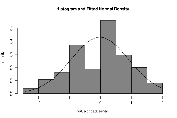
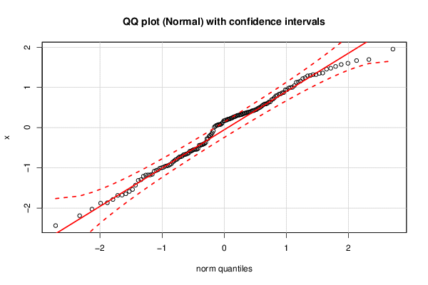
Title produced by software

ML Fitting and QQ Plot- Normal Distribution

Date of computation

Tue, 13 Oct 2015 14:32:43 +0100

Cite this page as follows

Statistical Computations at FreeStatistics.org, Office for Research Development and Education, URL https://freestatistics.org/blog/index.php?v=date/2015/Oct/13/t1444743173f84as6ij8uc7x8v.htm/, Retrieved Tue, 14 May 2024 03:07:36 +0000

Statistical Computations at FreeStatistics.org, Office for Research Development and Education, URL https://freestatistics.org/blog/index.php?pk=282353, Retrieved Tue, 14 May 2024 03:07:36 +0000

QR Codes:

Paste this QR Code to cite your computation.

Original text written by user:

IsPrivate?

No (this computation is public)

User-defined keywords

Estimated Impact

102

Family? (F = Feedback message, R = changed R code, M = changed R Module, P = changed Parameters, D = changed Data)

-       [ML Fitting and QQ Plot- Normal Distribution] [] [2015-10-13 13:32:43] [85e7a66a1e5d24b56c3cf5eab9332807] [Current]

Feedback Forum

Post a new message

Dataseries X:

Download CSV

Histogram

Boxplots

0.01415754875
-1.083993486
0.3944593523
0.8639702001
-0.6589151431
1.043060258
0.4880988084
0.3136258506
-1.537363433
0.4467293697
-0.9219617952
-0.6291306005
-0.7525579371
0.2407257079
-0.4290382375
-0.2189501052
0.5495727617
1.358828539
0.378832359
0.236842032
-0.7244410846
-0.5382548882
0.2905953829
0.8397941287
-0.4392188313
1.453345516
-1.046741652
-0.8287491186
-0.9447629866
-0.3937265195
-0.5376556265
-2.027348736
1.318682643
-0.7030686064
0.06172163103
-0.564798659
0.3251493743
1.349841007
1.952807553
0.09892213432
0.07683527763
-1.008621603
-0.7868524811
0.3610725537
-0.6726282562
0.4128846341
-1.175630644
-0.4060529484
-0.5855346497
0.9431509226
-2.190487676
0.8720487161
-0.7980860947
-0.1697209571
-0.5202689234
0.3086370126
-1.869001316
-0.367083228
0.7903749113
-0.9983495727
0.3812506172
0.220868116
-0.1935581362
0.5890047876
-0.8594079477
0.3850786228
0.2774077003
-1.586734335
0.9848533398
0.05699598515
0.3214302202
1.29569656
0.3666643216
1.137305158
1.218928051
-0.08031859676
-1.786278887
-1.065961385
-1.684464841
-1.176477286
0.6364275854
0.2100621643
0.03442946069
1.002614498
0.7449119694
-1.160065301
0.9980374658
-1.879010388
0.5754186472
0.07614400618
0.259112814
-0.6677568002
1.126074246
0.4247169487
0.6411909434
0.709830172
0.5020299645
0.130204782
0.18841767
1.286738296
0.169977607
0.2700436144
-0.2752463251
-1.295464236
-1.677958601
-0.5417104114
1.52255347
0.4717943544
0.3490445076
1.158729473
0.08051931368
0.8318871012
0.423150712
0.6073657839
-0.9889692553
1.240161039
0.1898811862
0.3442772356
-0.9631517745
-0.5495145219
-1.430494325
-1.645145869
-0.9028074932
0.2111744491
1.667809409
-1.179591366
-2.43680122
1.57028444
0.7962346069
1.478160255
-0.437254545
-1.209712162
1.601397106
0.590595829
-0.5853413446
-0.1278797547
0.3039779946
0.524205593
0.172291067
-1.311396379
-0.9530099258
0.9375926968
-0.7235239129
-0.272756064
-0.6465802836
-0.4210409257
1.317856971
0.4424042571
1.69324313
0.6929657089

Summary of computational transaction
Raw Input	view raw input (R code)
Raw Output	view raw output of R engine
Computing time	4 seconds
R Server	'Gertrude Mary Cox' @ cox.wessa.net

\begin{tabular}{lllllllll}
\hline
Summary of computational transaction \tabularnewline
Raw Input & view raw input (R code)  \tabularnewline
Raw Output & view raw output of R engine  \tabularnewline
Computing time & 4 seconds \tabularnewline
R Server & 'Gertrude Mary Cox' @ cox.wessa.net \tabularnewline
\hline
\end{tabular}
%Source: https://freestatistics.org/blog/index.php?pk=282353&T=0

[TABLE]
[ROW][C]Summary of computational transaction[/C][/ROW]
[ROW][C]Raw Input[/C][C]view raw input (R code) [/C][/ROW]
[ROW][C]Raw Output[/C][C]view raw output of R engine [/C][/ROW]
[ROW][C]Computing time[/C][C]4 seconds[/C][/ROW]
[ROW][C]R Server[/C][C]'Gertrude Mary Cox' @ cox.wessa.net[/C][/ROW]
[/TABLE]
Source: https://freestatistics.org/blog/index.php?pk=282353&T=0

Globally Unique Identifier (entire table): ba.freestatistics.org/blog/index.php?pk=282353&T=0

As an alternative you can also use a QR Code:

The GUIDs for individual cells are displayed in the table below:

Summary of computational transaction
Raw Input	view raw input (R code)
Raw Output	view raw output of R engine
Computing time	4 seconds
R Server	'Gertrude Mary Cox' @ cox.wessa.net

Parameter	Estimated Value	Standard Deviation
mean	-0.0201212679055333	0.075753525702136
standard deviation	0.92778742093522	0.0535658317227698

\begin{tabular}{lllllllll}
\hline
Parameter & Estimated Value & Standard Deviation \tabularnewline
mean & -0.0201212679055333 & 0.075753525702136 \tabularnewline
standard deviation & 0.92778742093522 & 0.0535658317227698 \tabularnewline
\hline
\end{tabular}
%Source: https://freestatistics.org/blog/index.php?pk=282353&T=1

[TABLE]
[ROW][C]Parameter[/C][C]Estimated Value[/C][C]Standard Deviation[/C][/ROW]
[ROW][C]mean[/C][C]-0.0201212679055333[/C][C]0.075753525702136[/C][/ROW]
[ROW][C]standard deviation[/C][C]0.92778742093522[/C][C]0.0535658317227698[/C][/ROW]
[/TABLE]
Source: https://freestatistics.org/blog/index.php?pk=282353&T=1

Globally Unique Identifier (entire table): ba.freestatistics.org/blog/index.php?pk=282353&T=1

As an alternative you can also use a QR Code:

The GUIDs for individual cells are displayed in the table below:

Parameter	Estimated Value	Standard Deviation
mean	-0.0201212679055333	0.075753525702136
standard deviation	0.92778742093522	0.0535658317227698

Figure 1

PNG link

Postscript link

PDF link

Figure 2

PNG link

Postscript link

PDF link

Parameters (Session):

par1 = 8 ; par2 = 0 ;

Parameters (R input):

par1 = 8 ; par2 = 0 ;

R code (references can be found in the software module):

library(MASS)
library(car)
par1 <- as.numeric(par1)
if (par2 == '0') par2 = 'Sturges' else par2 <- as.numeric(par2)
x <- as.ts(x) #otherwise the fitdistr function does not work properly
r <- fitdistr(x,'normal')
r
bitmap(file='test1.png')
myhist<-hist(x,col=par1,breaks=par2,main=main,ylab=ylab,xlab=xlab,freq=F)
curve(1/(r$estimate[2]*sqrt(2*pi))*exp(-1/2*((x-r$estimate[1])/r$estimate[2])^2),min(x),max(x),add=T)
dev.off()
bitmap(file='test3.png')
qqPlot(x,dist='norm',main='QQ plot (Normal) with confidence intervals')
grid()
dev.off()
load(file='createtable')
a<-table.start()
a<-table.row.start(a)
a<-table.element(a,'Parameter',1,TRUE)
a<-table.element(a,'Estimated Value',1,TRUE)
a<-table.element(a,'Standard Deviation',1,TRUE)
a<-table.row.end(a)
a<-table.row.start(a)
a<-table.element(a,'mean',header=TRUE)
a<-table.element(a,r$estimate[1])
a<-table.element(a,r$sd[1])
a<-table.row.end(a)
a<-table.row.start(a)
a<-table.element(a,'standard deviation',header=TRUE)
a<-table.element(a,r$estimate[2])
a<-table.element(a,r$sd[2])
a<-table.row.end(a)
a<-table.end(a)
table.save(a,file='mytable.tab')

Free Statistics

Description of Statistical Computation

Tree of Dependent Computations

Dataset

Tables (Output of Computation)

Figures (Output of Computation)

Input Parameters & R Code