Repository of Reproducible Computations

Free Statistics

of Irreproducible Research!

Author's title

Author

*The author of this computation has been verified*

R Software Module

rwasp_fitdistrnorm.wasp

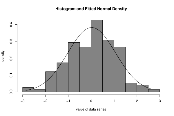
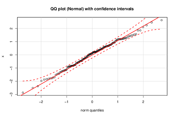
Title produced by software

ML Fitting and QQ Plot- Normal Distribution

Date of computation

Tue, 13 Oct 2015 15:49:23 +0100

Cite this page as follows

Statistical Computations at FreeStatistics.org, Office for Research Development and Education, URL https://freestatistics.org/blog/index.php?v=date/2015/Oct/13/t1444747791tadd3rcfu8iijdj.htm/, Retrieved Tue, 14 May 2024 02:09:37 +0000

Statistical Computations at FreeStatistics.org, Office for Research Development and Education, URL https://freestatistics.org/blog/index.php?pk=282367, Retrieved Tue, 14 May 2024 02:09:37 +0000

QR Codes:

Paste this QR Code to cite your computation.

Original text written by user:

IsPrivate?

No (this computation is public)

User-defined keywords

Estimated Impact

113

Family? (F = Feedback message, R = changed R code, M = changed R Module, P = changed Parameters, D = changed Data)

-       [ML Fitting and QQ Plot- Normal Distribution] [hoofdstuk 3:Task 3] [2015-10-13 14:49:23] [fdcee98729d8ae773847ef0dab21bb59] [Current]

Feedback Forum

Post a new message

Dataseries X:

Download CSV

Histogram

Boxplots

-1.521422685
-0.3690996767
0.2316457099
0.2117423917
-1.777602739
0.2689624432
1.201717155
-1.872837206
-0.5598515039
0.9388636075
0.3714513322
0.7747175539
0.1021277471
0.9000019935
1.17753904
-0.8719829471
-1.004760454
-2.858988377
-0.7438477721
-1.330735039
-1.155788583
1.418946598
-0.4749029506
0.6393807859
0.8546853974
0.2203408158
0.6878423951
-0.7900033656
0.6781830948
0.644142685
-0.8405768911
0.5773293743
-0.2010529543
0.2065244069
0.4142183401
-0.02207226534
1.342656288
1.567566688
-1.24439524
2.626294352
-1.692982575
1.179818322
0.5074851684
-1.425617101
0.2142300322
-0.1412691715
-2.372308651
-2.507030125
-1.814672055
1.274967867
-0.2567371012
-0.6250976675
-0.5636053483
-0.6314101555
0.6076001783
-0.8397809448
1.196654501
0.6851135452
-0.02050723781
-1.716851567
0.04843826291
-0.366553254
-0.07597714899
1.140979907
-1.310976006
0.6656975917
1.535343367
1.484811535
-0.885647079
-0.6211406221
-0.9186683985
-0.2678281513
-1.775379809
-0.4616299865
-1.429882897
0.2015166881
1.851740915
1.023546683
0.7384853809
0.2686018091
1.208690548
-0.3051048083
0.4621560657
-0.5552705416
0.7607211093
-0.8167052562
0.587936178
0.3768706405
-1.481548171
0.6010575862
1.187748628
-0.230337638
-1.247165002
0.1748633116
-0.7654645993
1.229279258
-0.8680032816
-1.199431531
-0.2999643529
-1.970818853
1.279952974
-0.4801084185
0.07443975037
-1.202265221
0.7572002171
0.9189720295
0.3079166433
1.12771106
1.463180994
2.4488052
1.174017931
2.107657025
0.4606253173
-0.3324484692
1.054955849
-0.2248569869
0.2217661003
0.404721679
0.1487566567
-0.5081153859
0.2964299317
1.847235592
0.098288893
-0.7592601845
0.402003209
-0.4526427134
0.04216688633
-1.15541888
0.9352727052
-0.6474955103
0.08752874352
-0.8929575238
-0.09385861132
1.256932997
0.2046900976
-1.124858416
0.2932193469
-0.824703583
-0.456327949
0.02377663273
0.8212896654
0.63808071
-0.8273953749
0.3620985939
-1.839350992
1.408913707
2.238005239
0.4617583426
0.5483237202
0.02374964871

Summary of computational transaction
Raw Input	view raw input (R code)
Raw Output	view raw output of R engine
Computing time	4 seconds
R Server	'Gwilym Jenkins' @ jenkins.wessa.net

\begin{tabular}{lllllllll}
\hline
Summary of computational transaction \tabularnewline
Raw Input & view raw input (R code)  \tabularnewline
Raw Output & view raw output of R engine  \tabularnewline
Computing time & 4 seconds \tabularnewline
R Server & 'Gwilym Jenkins' @ jenkins.wessa.net \tabularnewline
\hline
\end{tabular}
%Source: https://freestatistics.org/blog/index.php?pk=282367&T=0

[TABLE]
[ROW][C]Summary of computational transaction[/C][/ROW]
[ROW][C]Raw Input[/C][C]view raw input (R code) [/C][/ROW]
[ROW][C]Raw Output[/C][C]view raw output of R engine [/C][/ROW]
[ROW][C]Computing time[/C][C]4 seconds[/C][/ROW]
[ROW][C]R Server[/C][C]'Gwilym Jenkins' @ jenkins.wessa.net[/C][/ROW]
[/TABLE]
Source: https://freestatistics.org/blog/index.php?pk=282367&T=0

Globally Unique Identifier (entire table): ba.freestatistics.org/blog/index.php?pk=282367&T=0

As an alternative you can also use a QR Code:

The GUIDs for individual cells are displayed in the table below:

Summary of computational transaction
Raw Input	view raw input (R code)
Raw Output	view raw output of R engine
Computing time	4 seconds
R Server	'Gwilym Jenkins' @ jenkins.wessa.net

Parameter	Estimated Value	Standard Deviation
mean	0.0219221827027333	0.0852223104140242
standard deviation	1.04375587607718	0.0602612736021414

\begin{tabular}{lllllllll}
\hline
Parameter & Estimated Value & Standard Deviation \tabularnewline
mean & 0.0219221827027333 & 0.0852223104140242 \tabularnewline
standard deviation & 1.04375587607718 & 0.0602612736021414 \tabularnewline
\hline
\end{tabular}
%Source: https://freestatistics.org/blog/index.php?pk=282367&T=1

[TABLE]
[ROW][C]Parameter[/C][C]Estimated Value[/C][C]Standard Deviation[/C][/ROW]
[ROW][C]mean[/C][C]0.0219221827027333[/C][C]0.0852223104140242[/C][/ROW]
[ROW][C]standard deviation[/C][C]1.04375587607718[/C][C]0.0602612736021414[/C][/ROW]
[/TABLE]
Source: https://freestatistics.org/blog/index.php?pk=282367&T=1

Globally Unique Identifier (entire table): ba.freestatistics.org/blog/index.php?pk=282367&T=1

As an alternative you can also use a QR Code:

The GUIDs for individual cells are displayed in the table below:

Parameter	Estimated Value	Standard Deviation
mean	0.0219221827027333	0.0852223104140242
standard deviation	1.04375587607718	0.0602612736021414

Figure 1

PNG link

Postscript link

PDF link

Figure 2

PNG link

Postscript link

PDF link

Parameters (Session):

par1 = 8 ; par2 = 0 ;

Parameters (R input):

par1 = 8 ; par2 = 0 ;

R code (references can be found in the software module):

library(MASS)
library(car)
par1 <- as.numeric(par1)
if (par2 == '0') par2 = 'Sturges' else par2 <- as.numeric(par2)
x <- as.ts(x) #otherwise the fitdistr function does not work properly
r <- fitdistr(x,'normal')
r
bitmap(file='test1.png')
myhist<-hist(x,col=par1,breaks=par2,main=main,ylab=ylab,xlab=xlab,freq=F)
curve(1/(r$estimate[2]*sqrt(2*pi))*exp(-1/2*((x-r$estimate[1])/r$estimate[2])^2),min(x),max(x),add=T)
dev.off()
bitmap(file='test3.png')
qqPlot(x,dist='norm',main='QQ plot (Normal) with confidence intervals')
grid()
dev.off()
load(file='createtable')
a<-table.start()
a<-table.row.start(a)
a<-table.element(a,'Parameter',1,TRUE)
a<-table.element(a,'Estimated Value',1,TRUE)
a<-table.element(a,'Standard Deviation',1,TRUE)
a<-table.row.end(a)
a<-table.row.start(a)
a<-table.element(a,'mean',header=TRUE)
a<-table.element(a,r$estimate[1])
a<-table.element(a,r$sd[1])
a<-table.row.end(a)
a<-table.row.start(a)
a<-table.element(a,'standard deviation',header=TRUE)
a<-table.element(a,r$estimate[2])
a<-table.element(a,r$sd[2])
a<-table.row.end(a)
a<-table.end(a)
table.save(a,file='mytable.tab')

Free Statistics

Description of Statistical Computation

Tree of Dependent Computations

Dataset

Tables (Output of Computation)

Figures (Output of Computation)

Input Parameters & R Code