Free Statistics
of Irreproducible Research!
Description of Statistical Computation | |||||||||||||||||||||
|---|---|---|---|---|---|---|---|---|---|---|---|---|---|---|---|---|---|---|---|---|---|
| Author's title | |||||||||||||||||||||
| Author | *Unverified author* | ||||||||||||||||||||
| R Software Module | rwasp_meanplot.wasp | ||||||||||||||||||||
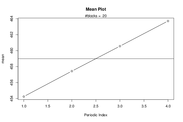
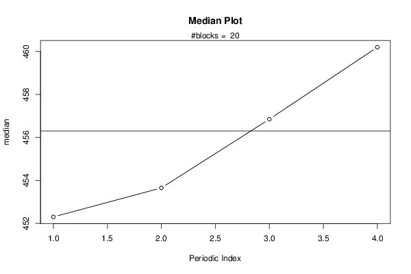
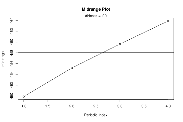
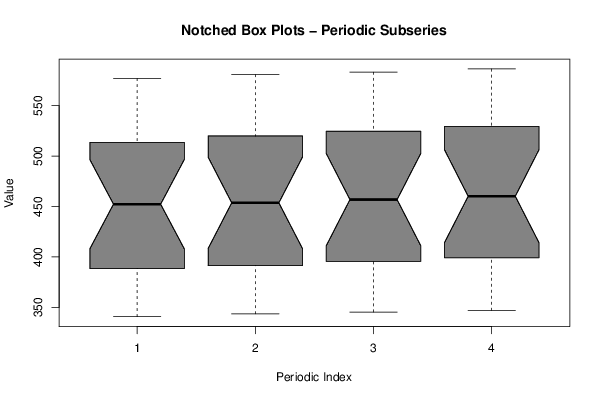
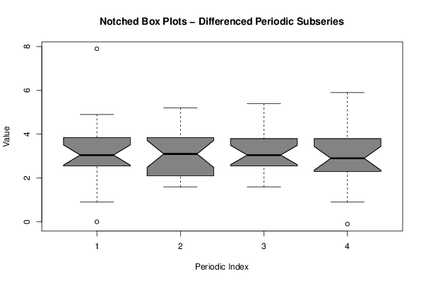
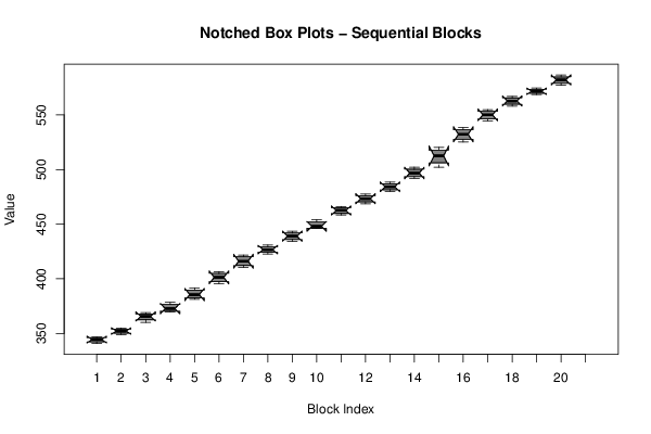
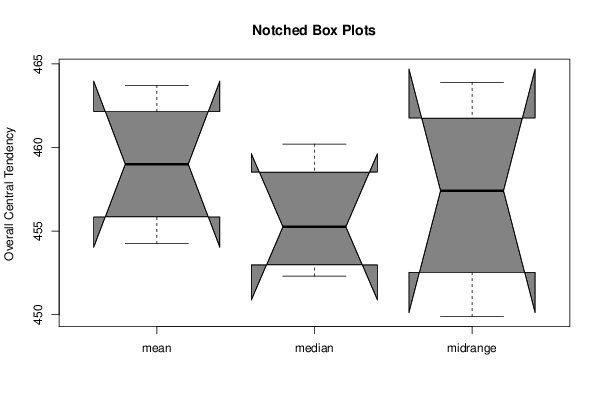
| Title produced by software | Mean Plot | ||||||||||||||||||||
| Date of computation | Sat, 17 Oct 2015 11:34:57 +0100 | ||||||||||||||||||||
| Cite this page as follows | Statistical Computations at FreeStatistics.org, Office for Research Development and Education, URL https://freestatistics.org/blog/index.php?v=date/2015/Oct/17/t1445078172q1npll8wxwzn1qh.htm/, Retrieved Wed, 15 May 2024 23:42:49 +0000 | ||||||||||||||||||||
| Statistical Computations at FreeStatistics.org, Office for Research Development and Education, URL https://freestatistics.org/blog/index.php?pk=282571, Retrieved Wed, 15 May 2024 23:42:49 +0000 | |||||||||||||||||||||
| QR Codes: | |||||||||||||||||||||
|
| |||||||||||||||||||||
| Original text written by user: | |||||||||||||||||||||
| IsPrivate? | No (this computation is public) | ||||||||||||||||||||
| User-defined keywords | |||||||||||||||||||||
| Estimated Impact | 132 | ||||||||||||||||||||
Tree of Dependent Computations | |||||||||||||||||||||
| Family? (F = Feedback message, R = changed R code, M = changed R Module, P = changed Parameters, D = changed Data) | |||||||||||||||||||||
| - [Mean Plot] [] [2015-10-17 10:34:57] [4535d628e97572fda841f25b347e529f] [Current] | |||||||||||||||||||||
| Feedback Forum | |||||||||||||||||||||
Post a new message | |||||||||||||||||||||
Dataset | |||||||||||||||||||||
| Dataseries X: | |||||||||||||||||||||
340,7 343,5 345,3 346,9 349 351,4 353 355 360,1 364,7 366,5 369 369,9 370,8 374,5 378,4 381,3 383,5 387,6 391,7 395,4 399,3 403,3 406,6 410,5 413,5 418,7 421,7 422,8 425,8 427,6 431 434,3 437,6 440,4 443,5 446,2 446,2 449,7 454,2 458,4 461,1 464 466,2 468,7 471,8 474,9 477,5 480 482,8 485,7 488,5 492 495,1 498,5 502,2 502,1 510 515 520,4 525,2 530,1 534,5 538,5 544,4 548,4 551,9 554,9 558,1 561,3 564,4 567 568,7 570,9 572,5 574,6 577,1 580,9 583,3 586,5 | |||||||||||||||||||||
Tables (Output of Computation) | |||||||||||||||||||||
| |||||||||||||||||||||
Figures (Output of Computation) | |||||||||||||||||||||
Input Parameters & R Code | |||||||||||||||||||||
| Parameters (Session): | |||||||||||||||||||||
| par1 = 4 ; | |||||||||||||||||||||
| Parameters (R input): | |||||||||||||||||||||
| par1 = 4 ; | |||||||||||||||||||||
| R code (references can be found in the software module): | |||||||||||||||||||||
par1 <- '12' | |||||||||||||||||||||