Free Statistics
of Irreproducible Research!
Description of Statistical Computation | |||||||||||||||||||||
|---|---|---|---|---|---|---|---|---|---|---|---|---|---|---|---|---|---|---|---|---|---|
| Author's title | |||||||||||||||||||||
| Author | *Unverified author* | ||||||||||||||||||||
| R Software Module | rwasp_meanplot.wasp | ||||||||||||||||||||
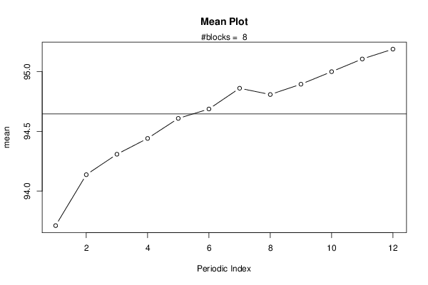
| Title produced by software | Mean Plot | ||||||||||||||||||||
| Date of computation | Fri, 23 Oct 2015 18:48:25 +0100 | ||||||||||||||||||||
| Cite this page as follows | Statistical Computations at FreeStatistics.org, Office for Research Development and Education, URL https://freestatistics.org/blog/index.php?v=date/2015/Oct/23/t144562252382h80jed96iip0o.htm/, Retrieved Tue, 14 May 2024 18:56:03 +0000 | ||||||||||||||||||||
| Statistical Computations at FreeStatistics.org, Office for Research Development and Education, URL https://freestatistics.org/blog/index.php?pk=282938, Retrieved Tue, 14 May 2024 18:56:03 +0000 | |||||||||||||||||||||
| QR Codes: | |||||||||||||||||||||
|
| |||||||||||||||||||||
| Original text written by user: | |||||||||||||||||||||
| IsPrivate? | No (this computation is public) | ||||||||||||||||||||
| User-defined keywords | |||||||||||||||||||||
| Estimated Impact | 75 | ||||||||||||||||||||
Tree of Dependent Computations | |||||||||||||||||||||
| Family? (F = Feedback message, R = changed R code, M = changed R Module, P = changed Parameters, D = changed Data) | |||||||||||||||||||||
| - [(Partial) Autocorrelation Function] [] [2015-10-23 17:29:21] [b1987693a2b63654c6d4ca246f63ea73] - P [(Partial) Autocorrelation Function] [] [2015-10-23 17:40:17] [b1987693a2b63654c6d4ca246f63ea73] - D [(Partial) Autocorrelation Function] [] [2015-10-23 17:45:59] [b1987693a2b63654c6d4ca246f63ea73] - RMPD [Mean Plot] [] [2015-10-23 17:48:25] [07f175c9375843c217f66b4a3796ae0c] [Current] | |||||||||||||||||||||
| Feedback Forum | |||||||||||||||||||||
Post a new message | |||||||||||||||||||||
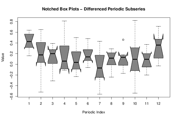
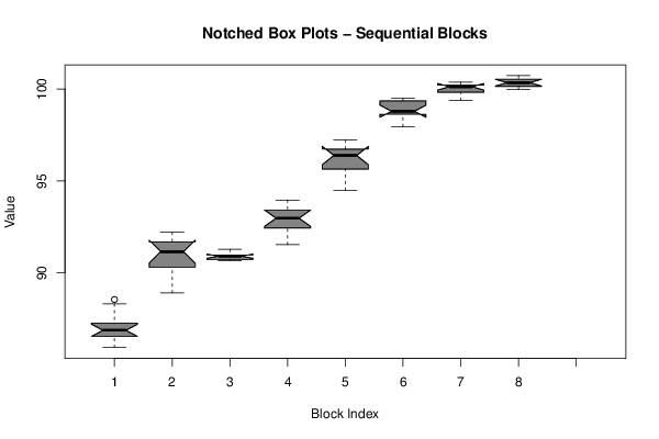
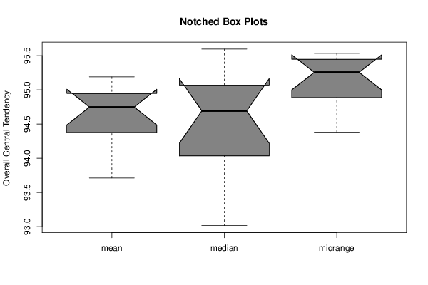
Dataset | |||||||||||||||||||||
| Dataseries X: | |||||||||||||||||||||
85.95 86.41 86.42 86.81 86.71 86.7 87.07 86.96 87.04 87.5 88.32 88.56 88.92 89.56 90.21 90.42 91.23 91.73 92.21 91.65 91.8 91.63 91.09 90.89 90.98 91.29 90.77 90.96 90.89 90.72 90.66 90.94 90.7 90.74 90.98 91.13 91.54 91.93 92.27 92.59 92.96 92.95 92.99 93.05 93.34 93.47 93.59 93.96 94.49 95.04 95.52 95.75 96.07 96.37 96.48 96.4 96.66 96.81 97.19 97.23 97.94 98.52 98.73 98.8 98.77 98.54 98.72 99.15 99.32 99.5 99.39 99.4 99.37 99.69 99.83 99.79 99.94 100.11 100.21 100.15 100.21 100.13 100.2 100.36 100.5 100.66 100.72 100.41 100.3 100.38 100.55 100.17 100.09 100.22 100.09 99.98 | |||||||||||||||||||||
Tables (Output of Computation) | |||||||||||||||||||||
| |||||||||||||||||||||
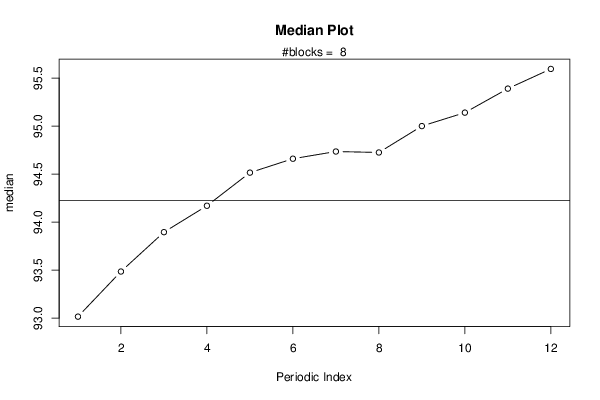
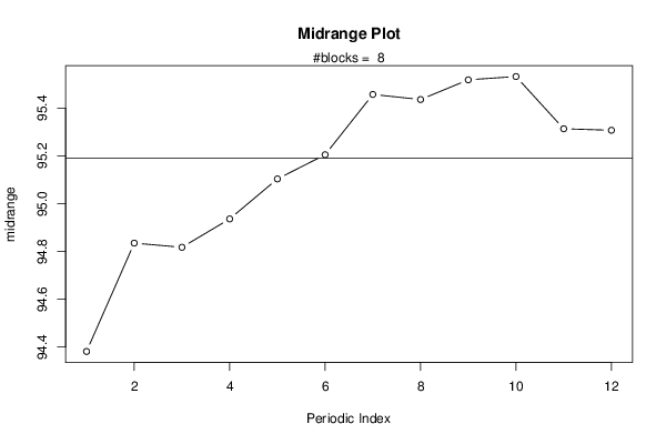
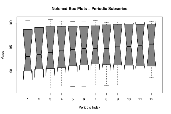
Figures (Output of Computation) | |||||||||||||||||||||
Input Parameters & R Code | |||||||||||||||||||||
| Parameters (Session): | |||||||||||||||||||||
| par1 = 12 ; | |||||||||||||||||||||
| Parameters (R input): | |||||||||||||||||||||
| par1 = 12 ; | |||||||||||||||||||||
| R code (references can be found in the software module): | |||||||||||||||||||||
par1 <- as.numeric(par1) | |||||||||||||||||||||