Free Statistics
of Irreproducible Research!
Description of Statistical Computation | ||||||||||||||||||||||||||||||||||||||||||||||||
|---|---|---|---|---|---|---|---|---|---|---|---|---|---|---|---|---|---|---|---|---|---|---|---|---|---|---|---|---|---|---|---|---|---|---|---|---|---|---|---|---|---|---|---|---|---|---|---|---|
| Author's title | ||||||||||||||||||||||||||||||||||||||||||||||||
| Author | *The author of this computation has been verified* | |||||||||||||||||||||||||||||||||||||||||||||||
| R Software Module | rwasp_fitdistrnorm.wasp | |||||||||||||||||||||||||||||||||||||||||||||||
| Title produced by software | ML Fitting and QQ Plot- Normal Distribution | |||||||||||||||||||||||||||||||||||||||||||||||
| Date of computation | Wed, 30 Nov 2016 11:49:44 +0100 | |||||||||||||||||||||||||||||||||||||||||||||||
| Cite this page as follows | Statistical Computations at FreeStatistics.org, Office for Research Development and Education, URL https://freestatistics.org/blog/index.php?v=date/2016/Nov/30/t1480503005y4hopjofrab7693.htm/, Retrieved Sat, 18 May 2024 20:42:40 +0000 | |||||||||||||||||||||||||||||||||||||||||||||||
| Statistical Computations at FreeStatistics.org, Office for Research Development and Education, URL https://freestatistics.org/blog/index.php?pk=297329, Retrieved Sat, 18 May 2024 20:42:40 +0000 | ||||||||||||||||||||||||||||||||||||||||||||||||
| QR Codes: | ||||||||||||||||||||||||||||||||||||||||||||||||
|
| ||||||||||||||||||||||||||||||||||||||||||||||||
| Original text written by user: | ||||||||||||||||||||||||||||||||||||||||||||||||
| IsPrivate? | No (this computation is public) | |||||||||||||||||||||||||||||||||||||||||||||||
| User-defined keywords | ||||||||||||||||||||||||||||||||||||||||||||||||
| Estimated Impact | 95 | |||||||||||||||||||||||||||||||||||||||||||||||
Tree of Dependent Computations | ||||||||||||||||||||||||||||||||||||||||||||||||
| Family? (F = Feedback message, R = changed R code, M = changed R Module, P = changed Parameters, D = changed Data) | ||||||||||||||||||||||||||||||||||||||||||||||||
| - [ML Fitting and QQ Plot- Normal Distribution] [] [2016-11-30 10:49:44] [94ac3c9a028ddd47e8862e80eac9f626] [Current] | ||||||||||||||||||||||||||||||||||||||||||||||||
| Feedback Forum | ||||||||||||||||||||||||||||||||||||||||||||||||
Post a new message | ||||||||||||||||||||||||||||||||||||||||||||||||
Dataset | ||||||||||||||||||||||||||||||||||||||||||||||||
| Dataseries X: | ||||||||||||||||||||||||||||||||||||||||||||||||
-35.68 -39.41 -90.98 -99.79 9.899 -55.35 -82.98 -26.85 -130.7 -196 103.4 -17.23 29.32 217.6 119 73.21 -47.1 -46.35 163 143.1 9.336 159 193.4 312.8 307.3 107.6 95.02 138.2 182.9 179.6 153 269.1 -90.66 143 184.4 26.77 357.3 220.6 237 84.21 353.9 286.6 323 32.15 68.34 127 348.4 488.8 374.3 415.6 79.02 456.2 380.9 246.6 370 255.1 374.3 231 69.4 -15.23 -114.7 -44.41 -49.98 -102.8 108.9 231.6 137 230.1 294.3 228 43.4 -114.2 -145.7 -191.4 54.02 -102.8 -103.1 -145.4 -200 -113.9 -53.66 -288 -143.6 33.77 -249.7 107.6 -191 -89.79 -92.1 -257.4 -116 -329.9 -82.66 -101 -90.6 108.8 -74.68 -146.4 -187 -81.79 -228.1 -46.35 -114 -13.85 -194.7 -164 -48.6 49.77 233.3 -85.41 -34.98 -25.79 -176.1 55.65 15.02 -18.85 -66.66 -166 1.399 96.77 90.32 -102.4 164 -23.79 -66.1 -135.4 -215 -102.9 -64.66 -196 -32.6 41.77 -57.68 -186.4 -91.98 -124.8 -169.1 -44.35 -182 -104.9 -161.7 -22.04 -311.6 -224.2 -248.7 -89.41 -55.98 -80.79 -100.1 -181.4 -0.9764 -146.9 -28.66 88.96 -180.6 -439.2 -266.7 -102.4 -142 -119.8 -135.1 -8.351 -154 27.15 -115.7 0.9611 -50.6 -86.23 -228.7 -94.6 15.83 79.02 9.71 -94.54 -72.17 -122 113.1 33.77 -169.8 -256.4 30.14 13.4 79.83 21.02 70.71 14.46 -24.17 22.96 130.1 121.8 84.21 -6.415 | ||||||||||||||||||||||||||||||||||||||||||||||||
Tables (Output of Computation) | ||||||||||||||||||||||||||||||||||||||||||||||||
| ||||||||||||||||||||||||||||||||||||||||||||||||
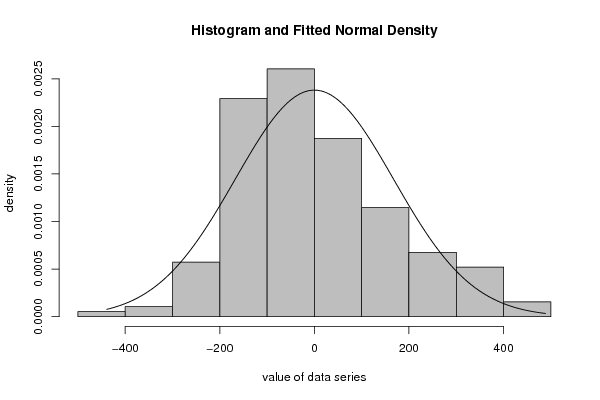
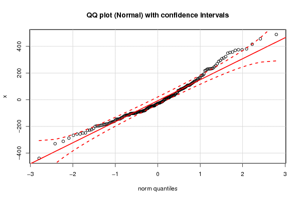
Figures (Output of Computation) | ||||||||||||||||||||||||||||||||||||||||||||||||
Input Parameters & R Code | ||||||||||||||||||||||||||||||||||||||||||||||||
| Parameters (Session): | ||||||||||||||||||||||||||||||||||||||||||||||||
| par1 = 8 ; par2 = 0 ; | ||||||||||||||||||||||||||||||||||||||||||||||||
| Parameters (R input): | ||||||||||||||||||||||||||||||||||||||||||||||||
| par1 = 8 ; par2 = 0 ; | ||||||||||||||||||||||||||||||||||||||||||||||||
| R code (references can be found in the software module): | ||||||||||||||||||||||||||||||||||||||||||||||||
library(MASS) | ||||||||||||||||||||||||||||||||||||||||||||||||