Free Statistics
of Irreproducible Research!
Description of Statistical Computation | ||||||||||||||||||||||||||||||
|---|---|---|---|---|---|---|---|---|---|---|---|---|---|---|---|---|---|---|---|---|---|---|---|---|---|---|---|---|---|---|
| Author's title | ||||||||||||||||||||||||||||||
| Author | *Unverified author* | |||||||||||||||||||||||||||||
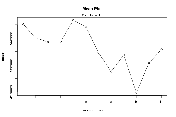
| R Software Module | rwasp_meanplot.wasp | |||||||||||||||||||||||||||||
| Title produced by software | Mean Plot | |||||||||||||||||||||||||||||
| Date of computation | Sun, 06 Aug 2017 17:40:51 +0200 | |||||||||||||||||||||||||||||
| Cite this page as follows | Statistical Computations at FreeStatistics.org, Office for Research Development and Education, URL https://freestatistics.org/blog/index.php?v=date/2017/Aug/06/t1502034070oyv2xowa8x0z3o4.htm/, Retrieved Sun, 12 May 2024 07:52:12 +0000 | |||||||||||||||||||||||||||||
| Statistical Computations at FreeStatistics.org, Office for Research Development and Education, URL https://freestatistics.org/blog/index.php?pk=306960, Retrieved Sun, 12 May 2024 07:52:12 +0000 | ||||||||||||||||||||||||||||||
| QR Codes: | ||||||||||||||||||||||||||||||
|
| ||||||||||||||||||||||||||||||
| Original text written by user: | ||||||||||||||||||||||||||||||
| IsPrivate? | No (this computation is public) | |||||||||||||||||||||||||||||
| User-defined keywords | ||||||||||||||||||||||||||||||
| Estimated Impact | 127 | |||||||||||||||||||||||||||||
Tree of Dependent Computations | ||||||||||||||||||||||||||||||
| Family? (F = Feedback message, R = changed R code, M = changed R Module, P = changed Parameters, D = changed Data) | ||||||||||||||||||||||||||||||
| - [Mean Plot] [] [2017-08-06 15:40:51] [bb1ebaef39f3ee233240b5c77a617fca] [Current] | ||||||||||||||||||||||||||||||
| Feedback Forum | ||||||||||||||||||||||||||||||
Post a new message | ||||||||||||||||||||||||||||||
Dataset | ||||||||||||||||||||||||||||||
| Dataseries X: | ||||||||||||||||||||||||||||||
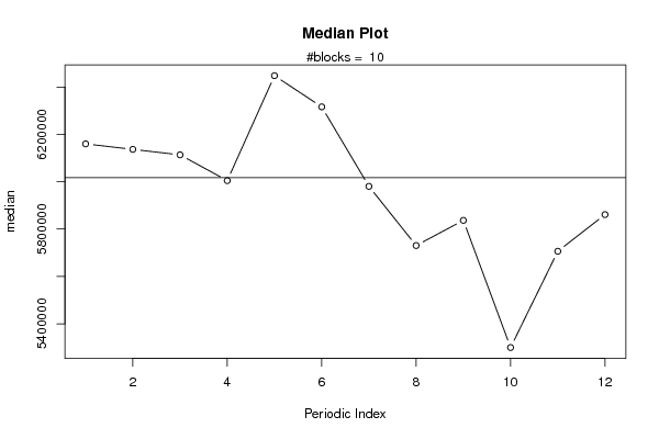
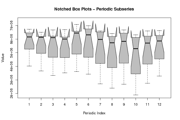
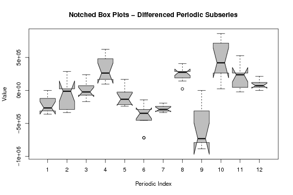
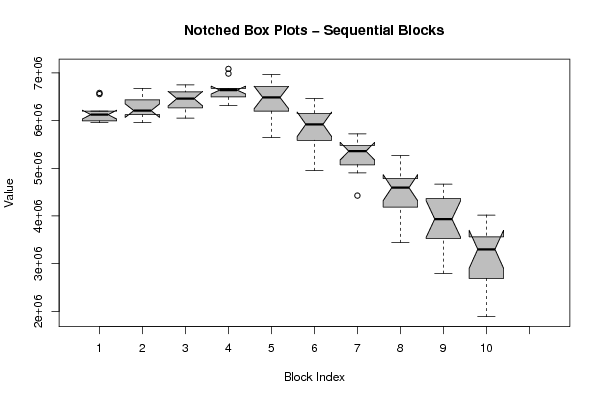
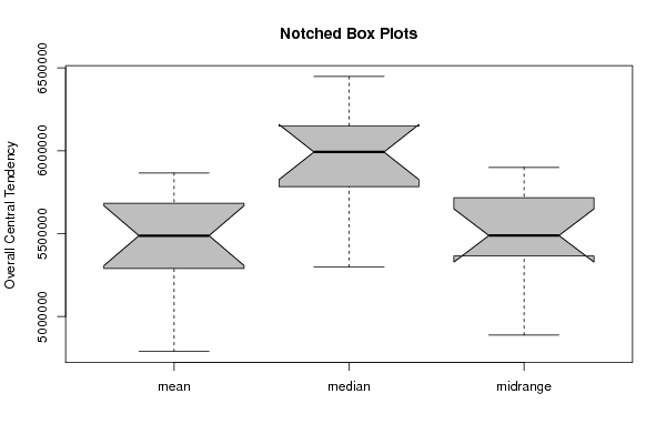
6195800,00 6172725,00 6149325,00 6100900,00 6579950,00 6554600,00 6195800,00 5957250,00 5980325,00 5980325,00 6006000,00 6052150,00 6123975,00 6123975,00 6077825,00 5957250,00 6579950,00 6674850,00 6531525,00 6195800,00 6339450,00 6123975,00 6221150,00 6267625,00 6316050,00 6195800,00 6221150,00 6052150,00 6579950,00 6746675,00 6603350,00 6339450,00 6626425,00 6316050,00 6603350,00 6579950,00 6651775,00 6387875,00 6674850,00 6651775,00 7082400,00 6985225,00 6603350,00 6410950,00 6674850,00 6316050,00 6579950,00 6626425,00 6723600,00 6508450,00 6626425,00 6698250,00 6962150,00 6746675,00 6459700,00 6149325,00 6436625,00 5646875,00 6029075,00 6244225,00 6459700,00 6149325,00 6149325,00 6149325,00 6316050,00 6077825,00 5765175,00 5503550,00 5693350,00 4952350,00 5406375,00 5670275,00 5718700,00 5454800,00 5477875,00 5406375,00 5646875,00 5477875,00 5144750,00 4903925,00 5311150,00 4426825,00 5001100,00 5262725,00 5262725,00 4952350,00 4665375,00 4642300,00 4903925,00 4665375,00 4211675,00 3899025,00 4234750,00 3445325,00 4162925,00 4544800,00 4665375,00 4401475,00 4068025,00 4306575,00 4401475,00 4329650,00 3611725,00 3278600,00 3516825,00 2799225,00 3540225,00 3804125,00 4019275,00 3660475,00 3324750,00 3516825,00 3611725,00 3421925,00 2704325,00 2391675,00 2678650,00 1889225,00 2750475,00 3278600,00 | ||||||||||||||||||||||||||||||
Tables (Output of Computation) | ||||||||||||||||||||||||||||||
| ||||||||||||||||||||||||||||||
Figures (Output of Computation) | ||||||||||||||||||||||||||||||
Input Parameters & R Code | ||||||||||||||||||||||||||||||
| Parameters (Session): | ||||||||||||||||||||||||||||||
| Parameters (R input): | ||||||||||||||||||||||||||||||
| par1 = 12 ; | ||||||||||||||||||||||||||||||
| R code (references can be found in the software module): | ||||||||||||||||||||||||||||||
par1 <- as.numeric(par1) | ||||||||||||||||||||||||||||||