Repository of Reproducible Computations

Free Statistics

of Irreproducible Research!

Author's title

Author

*Unverified author*

R Software Module

rwasp_decompose.wasp

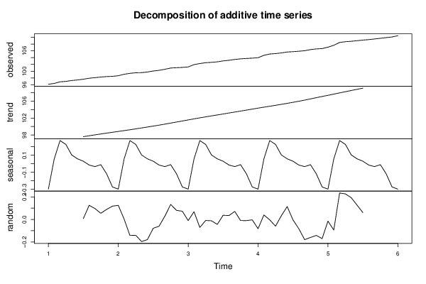
Title produced by software

Classical Decomposition

Date of computation

Mon, 01 May 2017 10:43:03 +0100

Cite this page as follows

Statistical Computations at FreeStatistics.org, Office for Research Development and Education, URL https://freestatistics.org/blog/index.php?v=date/2017/May/01/t1493631811ybkdee0ug8ocgqk.htm/, Retrieved Mon, 27 May 2024 07:44:42 +0200

Statistical Computations at FreeStatistics.org, Office for Research Development and Education, URL https://freestatistics.org/blog/index.php?pk=, Retrieved Mon, 27 May 2024 07:44:42 +0200

QR Codes:

Paste this QR Code to cite your computation.

Original text written by user:

IsPrivate?

No (this computation is public)

User-defined keywords

Estimated Impact

Dataseries X:

Download CSV

Histogram

Boxplots

Summary of computational transaction
Raw Input	view raw input (R code)
Raw Output	view raw output of R engine
Computing time	3 seconds
R Server	'Gwilym Jenkins' @ jenkins.wessa.net

\begin{tabular}{lllllllll}
\hline
Summary of computational transaction \tabularnewline
Raw Input & view raw input (R code)  \tabularnewline
Raw Output & view raw output of R engine  \tabularnewline
Computing time & 3 seconds \tabularnewline
R Server & 'Gwilym Jenkins' @ jenkins.wessa.net \tabularnewline
\hline
\end{tabular}
%Source: https://freestatistics.org/blog/index.php?pk=&T=0

[TABLE]
[ROW][C]Summary of computational transaction[/C][/ROW]
[ROW][C]Raw Input[/C][C]view raw input (R code) [/C][/ROW]
[ROW][C]Raw Output[/C][C]view raw output of R engine [/C][/ROW]
[ROW][C]Computing time[/C][C]3 seconds[/C][/ROW]
[ROW][C]R Server[/C][C]'Gwilym Jenkins' @ jenkins.wessa.net[/C][/ROW]
[/TABLE]
Source: https://freestatistics.org/blog/index.php?pk=&T=0

Globally Unique Identifier (entire table): ba.freestatistics.org/blog/index.php?pk=&T=0

As an alternative you can also use a QR Code:

The GUIDs for individual cells are displayed in the table below:

Summary of computational transaction
Raw Input	view raw input (R code)
Raw Output	view raw output of R engine
Computing time	3 seconds
R Server	'Gwilym Jenkins' @ jenkins.wessa.net

Classical Decomposition by Moving Averages
t	Observations	Fit	Trend	Seasonal	Random
1	96.16	NA	NA	-0.297215	NA
2	96.4	NA	NA	0.0565347	NA
3	96.87	NA	NA	0.271743	NA
4	97	NA	NA	0.226639	NA
5	97.26	NA	NA	0.103201	NA
6	97.42	NA	NA	0.0577847	NA
7	97.64	97.6327	97.6029	0.0297847	0.00729861
8	97.93	97.8049	97.82	-0.0151319	0.125132
9	98.1	98.0036	98.0367	-0.0330486	0.0963819
10	98.29	98.2359	98.2467	-0.0107569	0.0540903
11	98.42	98.3311	98.4492	-0.118049	0.0888819
12	98.49	98.3723	98.6438	-0.271486	0.117736
13	98.67	98.5453	98.8425	-0.297215	0.124715
14	99.1	99.097	99.0404	0.0565347	0.00304861
15	99.37	99.5122	99.2404	0.271743	-0.14216
16	99.54	99.6804	99.4537	0.226639	-0.140389
17	99.58	99.7761	99.6729	0.103201	-0.196118
18	99.77	99.949	99.8912	0.0577847	-0.179035
19	100.06	100.139	100.109	0.0297847	-0.0785347
20	100.26	100.32	100.335	-0.0151319	-0.0598681
21	100.57	100.541	100.574	-0.0330486	0.0292986
22	100.94	100.807	100.818	-0.0107569	0.13284
23	101.03	100.95	101.068	-0.118049	0.0801319
24	101.12	101.047	101.319	-0.271486	0.0727361
25	101.26	101.27	101.568	-0.297215	-0.0102847
26	101.94	101.872	101.815	0.0565347	0.0684653
27	102.26	102.331	102.059	0.271743	-0.0709097
28	102.51	102.519	102.292	0.226639	-0.00913889
29	102.61	102.622	102.519	0.103201	-0.0119514
30	102.76	102.804	102.746	0.0577847	-0.0440347
31	103.04	103.003	102.973	0.0297847	0.0368819
32	103.22	103.186	103.201	-0.0151319	0.0342986
33	103.47	103.399	103.432	-0.0330486	0.0709653
34	103.64	103.65	103.661	-0.0107569	-0.0100764
35	103.76	103.77	103.888	-0.118049	-0.0102847
36	103.85	103.854	104.125	-0.271486	-0.00351389
37	103.98	104.062	104.359	-0.297215	-0.0819514
38	104.68	104.64	104.584	0.0565347	0.0397153
39	105.07	105.074	104.802	0.271743	-0.00382639
40	105.19	105.25	105.023	0.226639	-0.0595556
41	105.39	105.357	105.254	0.103201	0.0330486
42	105.66	105.546	105.488	0.0577847	0.113882
43	105.76	105.765	105.735	0.0297847	-0.00478472
44	105.89	105.972	105.987	-0.0151319	-0.0823681
45	106.04	106.219	106.252	-0.0330486	-0.179451
46	106.37	106.53	106.54	-0.0107569	-0.15966
47	106.57	106.712	106.83	-0.118049	-0.141535
48	106.67	106.84	107.111	-0.271486	-0.169764
49	107.08	107.095	107.392	-0.297215	-0.0152847
50	107.64	107.734	107.677	0.0565347	-0.0940347
51	108.47	108.236	107.964	0.271743	0.23409
52	108.7	108.474	108.247	0.226639	0.226278
53	108.82	108.628	108.525	0.103201	0.192215
54	108.99	108.864	108.806	0.0577847	0.126382
55	109.18	109.119	109.09	0.0297847	0.0606319
56	109.31	NA	NA	-0.0151319	NA
57	109.5	NA	NA	-0.0330486	NA
58	109.7	NA	NA	-0.0107569	NA
59	109.9	NA	NA	-0.118049	NA
60	110.09	NA	NA	-0.271486	NA
61	110.47	NA	NA	-0.297215	NA

\begin{tabular}{lllllllll}
\hline
Classical Decomposition by Moving Averages \tabularnewline
t & Observations & Fit & Trend & Seasonal & Random \tabularnewline
1 & 96.16 & NA & NA & -0.297215 & NA \tabularnewline
2 & 96.4 & NA & NA & 0.0565347 & NA \tabularnewline
3 & 96.87 & NA & NA & 0.271743 & NA \tabularnewline
4 & 97 & NA & NA & 0.226639 & NA \tabularnewline
5 & 97.26 & NA & NA & 0.103201 & NA \tabularnewline
6 & 97.42 & NA & NA & 0.0577847 & NA \tabularnewline
7 & 97.64 & 97.6327 & 97.6029 & 0.0297847 & 0.00729861 \tabularnewline
8 & 97.93 & 97.8049 & 97.82 & -0.0151319 & 0.125132 \tabularnewline
9 & 98.1 & 98.0036 & 98.0367 & -0.0330486 & 0.0963819 \tabularnewline
10 & 98.29 & 98.2359 & 98.2467 & -0.0107569 & 0.0540903 \tabularnewline
11 & 98.42 & 98.3311 & 98.4492 & -0.118049 & 0.0888819 \tabularnewline
12 & 98.49 & 98.3723 & 98.6438 & -0.271486 & 0.117736 \tabularnewline
13 & 98.67 & 98.5453 & 98.8425 & -0.297215 & 0.124715 \tabularnewline
14 & 99.1 & 99.097 & 99.0404 & 0.0565347 & 0.00304861 \tabularnewline
15 & 99.37 & 99.5122 & 99.2404 & 0.271743 & -0.14216 \tabularnewline
16 & 99.54 & 99.6804 & 99.4537 & 0.226639 & -0.140389 \tabularnewline
17 & 99.58 & 99.7761 & 99.6729 & 0.103201 & -0.196118 \tabularnewline
18 & 99.77 & 99.949 & 99.8912 & 0.0577847 & -0.179035 \tabularnewline
19 & 100.06 & 100.139 & 100.109 & 0.0297847 & -0.0785347 \tabularnewline
20 & 100.26 & 100.32 & 100.335 & -0.0151319 & -0.0598681 \tabularnewline
21 & 100.57 & 100.541 & 100.574 & -0.0330486 & 0.0292986 \tabularnewline
22 & 100.94 & 100.807 & 100.818 & -0.0107569 & 0.13284 \tabularnewline
23 & 101.03 & 100.95 & 101.068 & -0.118049 & 0.0801319 \tabularnewline
24 & 101.12 & 101.047 & 101.319 & -0.271486 & 0.0727361 \tabularnewline
25 & 101.26 & 101.27 & 101.568 & -0.297215 & -0.0102847 \tabularnewline
26 & 101.94 & 101.872 & 101.815 & 0.0565347 & 0.0684653 \tabularnewline
27 & 102.26 & 102.331 & 102.059 & 0.271743 & -0.0709097 \tabularnewline
28 & 102.51 & 102.519 & 102.292 & 0.226639 & -0.00913889 \tabularnewline
29 & 102.61 & 102.622 & 102.519 & 0.103201 & -0.0119514 \tabularnewline
30 & 102.76 & 102.804 & 102.746 & 0.0577847 & -0.0440347 \tabularnewline
31 & 103.04 & 103.003 & 102.973 & 0.0297847 & 0.0368819 \tabularnewline
32 & 103.22 & 103.186 & 103.201 & -0.0151319 & 0.0342986 \tabularnewline
33 & 103.47 & 103.399 & 103.432 & -0.0330486 & 0.0709653 \tabularnewline
34 & 103.64 & 103.65 & 103.661 & -0.0107569 & -0.0100764 \tabularnewline
35 & 103.76 & 103.77 & 103.888 & -0.118049 & -0.0102847 \tabularnewline
36 & 103.85 & 103.854 & 104.125 & -0.271486 & -0.00351389 \tabularnewline
37 & 103.98 & 104.062 & 104.359 & -0.297215 & -0.0819514 \tabularnewline
38 & 104.68 & 104.64 & 104.584 & 0.0565347 & 0.0397153 \tabularnewline
39 & 105.07 & 105.074 & 104.802 & 0.271743 & -0.00382639 \tabularnewline
40 & 105.19 & 105.25 & 105.023 & 0.226639 & -0.0595556 \tabularnewline
41 & 105.39 & 105.357 & 105.254 & 0.103201 & 0.0330486 \tabularnewline
42 & 105.66 & 105.546 & 105.488 & 0.0577847 & 0.113882 \tabularnewline
43 & 105.76 & 105.765 & 105.735 & 0.0297847 & -0.00478472 \tabularnewline
44 & 105.89 & 105.972 & 105.987 & -0.0151319 & -0.0823681 \tabularnewline
45 & 106.04 & 106.219 & 106.252 & -0.0330486 & -0.179451 \tabularnewline
46 & 106.37 & 106.53 & 106.54 & -0.0107569 & -0.15966 \tabularnewline
47 & 106.57 & 106.712 & 106.83 & -0.118049 & -0.141535 \tabularnewline
48 & 106.67 & 106.84 & 107.111 & -0.271486 & -0.169764 \tabularnewline
49 & 107.08 & 107.095 & 107.392 & -0.297215 & -0.0152847 \tabularnewline
50 & 107.64 & 107.734 & 107.677 & 0.0565347 & -0.0940347 \tabularnewline
51 & 108.47 & 108.236 & 107.964 & 0.271743 & 0.23409 \tabularnewline
52 & 108.7 & 108.474 & 108.247 & 0.226639 & 0.226278 \tabularnewline
53 & 108.82 & 108.628 & 108.525 & 0.103201 & 0.192215 \tabularnewline
54 & 108.99 & 108.864 & 108.806 & 0.0577847 & 0.126382 \tabularnewline
55 & 109.18 & 109.119 & 109.09 & 0.0297847 & 0.0606319 \tabularnewline
56 & 109.31 & NA & NA & -0.0151319 & NA \tabularnewline
57 & 109.5 & NA & NA & -0.0330486 & NA \tabularnewline
58 & 109.7 & NA & NA & -0.0107569 & NA \tabularnewline
59 & 109.9 & NA & NA & -0.118049 & NA \tabularnewline
60 & 110.09 & NA & NA & -0.271486 & NA \tabularnewline
61 & 110.47 & NA & NA & -0.297215 & NA \tabularnewline
\hline
\end{tabular}
%Source: https://freestatistics.org/blog/index.php?pk=&T=1

[TABLE]
[ROW][C]Classical Decomposition by Moving Averages[/C][/ROW]
[ROW][C]t[/C][C]Observations[/C][C]Fit[/C][C]Trend[/C][C]Seasonal[/C][C]Random[/C][/ROW]
[ROW][C]1[/C][C]96.16[/C][C]NA[/C][C]NA[/C][C]-0.297215[/C][C]NA[/C][/ROW]
[ROW][C]2[/C][C]96.4[/C][C]NA[/C][C]NA[/C][C]0.0565347[/C][C]NA[/C][/ROW]
[ROW][C]3[/C][C]96.87[/C][C]NA[/C][C]NA[/C][C]0.271743[/C][C]NA[/C][/ROW]
[ROW][C]4[/C][C]97[/C][C]NA[/C][C]NA[/C][C]0.226639[/C][C]NA[/C][/ROW]
[ROW][C]5[/C][C]97.26[/C][C]NA[/C][C]NA[/C][C]0.103201[/C][C]NA[/C][/ROW]
[ROW][C]6[/C][C]97.42[/C][C]NA[/C][C]NA[/C][C]0.0577847[/C][C]NA[/C][/ROW]
[ROW][C]7[/C][C]97.64[/C][C]97.6327[/C][C]97.6029[/C][C]0.0297847[/C][C]0.00729861[/C][/ROW]
[ROW][C]8[/C][C]97.93[/C][C]97.8049[/C][C]97.82[/C][C]-0.0151319[/C][C]0.125132[/C][/ROW]
[ROW][C]9[/C][C]98.1[/C][C]98.0036[/C][C]98.0367[/C][C]-0.0330486[/C][C]0.0963819[/C][/ROW]
[ROW][C]10[/C][C]98.29[/C][C]98.2359[/C][C]98.2467[/C][C]-0.0107569[/C][C]0.0540903[/C][/ROW]
[ROW][C]11[/C][C]98.42[/C][C]98.3311[/C][C]98.4492[/C][C]-0.118049[/C][C]0.0888819[/C][/ROW]
[ROW][C]12[/C][C]98.49[/C][C]98.3723[/C][C]98.6438[/C][C]-0.271486[/C][C]0.117736[/C][/ROW]
[ROW][C]13[/C][C]98.67[/C][C]98.5453[/C][C]98.8425[/C][C]-0.297215[/C][C]0.124715[/C][/ROW]
[ROW][C]14[/C][C]99.1[/C][C]99.097[/C][C]99.0404[/C][C]0.0565347[/C][C]0.00304861[/C][/ROW]
[ROW][C]15[/C][C]99.37[/C][C]99.5122[/C][C]99.2404[/C][C]0.271743[/C][C]-0.14216[/C][/ROW]
[ROW][C]16[/C][C]99.54[/C][C]99.6804[/C][C]99.4537[/C][C]0.226639[/C][C]-0.140389[/C][/ROW]
[ROW][C]17[/C][C]99.58[/C][C]99.7761[/C][C]99.6729[/C][C]0.103201[/C][C]-0.196118[/C][/ROW]
[ROW][C]18[/C][C]99.77[/C][C]99.949[/C][C]99.8912[/C][C]0.0577847[/C][C]-0.179035[/C][/ROW]
[ROW][C]19[/C][C]100.06[/C][C]100.139[/C][C]100.109[/C][C]0.0297847[/C][C]-0.0785347[/C][/ROW]
[ROW][C]20[/C][C]100.26[/C][C]100.32[/C][C]100.335[/C][C]-0.0151319[/C][C]-0.0598681[/C][/ROW]
[ROW][C]21[/C][C]100.57[/C][C]100.541[/C][C]100.574[/C][C]-0.0330486[/C][C]0.0292986[/C][/ROW]
[ROW][C]22[/C][C]100.94[/C][C]100.807[/C][C]100.818[/C][C]-0.0107569[/C][C]0.13284[/C][/ROW]
[ROW][C]23[/C][C]101.03[/C][C]100.95[/C][C]101.068[/C][C]-0.118049[/C][C]0.0801319[/C][/ROW]
[ROW][C]24[/C][C]101.12[/C][C]101.047[/C][C]101.319[/C][C]-0.271486[/C][C]0.0727361[/C][/ROW]
[ROW][C]25[/C][C]101.26[/C][C]101.27[/C][C]101.568[/C][C]-0.297215[/C][C]-0.0102847[/C][/ROW]
[ROW][C]26[/C][C]101.94[/C][C]101.872[/C][C]101.815[/C][C]0.0565347[/C][C]0.0684653[/C][/ROW]
[ROW][C]27[/C][C]102.26[/C][C]102.331[/C][C]102.059[/C][C]0.271743[/C][C]-0.0709097[/C][/ROW]
[ROW][C]28[/C][C]102.51[/C][C]102.519[/C][C]102.292[/C][C]0.226639[/C][C]-0.00913889[/C][/ROW]
[ROW][C]29[/C][C]102.61[/C][C]102.622[/C][C]102.519[/C][C]0.103201[/C][C]-0.0119514[/C][/ROW]
[ROW][C]30[/C][C]102.76[/C][C]102.804[/C][C]102.746[/C][C]0.0577847[/C][C]-0.0440347[/C][/ROW]
[ROW][C]31[/C][C]103.04[/C][C]103.003[/C][C]102.973[/C][C]0.0297847[/C][C]0.0368819[/C][/ROW]
[ROW][C]32[/C][C]103.22[/C][C]103.186[/C][C]103.201[/C][C]-0.0151319[/C][C]0.0342986[/C][/ROW]
[ROW][C]33[/C][C]103.47[/C][C]103.399[/C][C]103.432[/C][C]-0.0330486[/C][C]0.0709653[/C][/ROW]
[ROW][C]34[/C][C]103.64[/C][C]103.65[/C][C]103.661[/C][C]-0.0107569[/C][C]-0.0100764[/C][/ROW]
[ROW][C]35[/C][C]103.76[/C][C]103.77[/C][C]103.888[/C][C]-0.118049[/C][C]-0.0102847[/C][/ROW]
[ROW][C]36[/C][C]103.85[/C][C]103.854[/C][C]104.125[/C][C]-0.271486[/C][C]-0.00351389[/C][/ROW]
[ROW][C]37[/C][C]103.98[/C][C]104.062[/C][C]104.359[/C][C]-0.297215[/C][C]-0.0819514[/C][/ROW]
[ROW][C]38[/C][C]104.68[/C][C]104.64[/C][C]104.584[/C][C]0.0565347[/C][C]0.0397153[/C][/ROW]
[ROW][C]39[/C][C]105.07[/C][C]105.074[/C][C]104.802[/C][C]0.271743[/C][C]-0.00382639[/C][/ROW]
[ROW][C]40[/C][C]105.19[/C][C]105.25[/C][C]105.023[/C][C]0.226639[/C][C]-0.0595556[/C][/ROW]
[ROW][C]41[/C][C]105.39[/C][C]105.357[/C][C]105.254[/C][C]0.103201[/C][C]0.0330486[/C][/ROW]
[ROW][C]42[/C][C]105.66[/C][C]105.546[/C][C]105.488[/C][C]0.0577847[/C][C]0.113882[/C][/ROW]
[ROW][C]43[/C][C]105.76[/C][C]105.765[/C][C]105.735[/C][C]0.0297847[/C][C]-0.00478472[/C][/ROW]
[ROW][C]44[/C][C]105.89[/C][C]105.972[/C][C]105.987[/C][C]-0.0151319[/C][C]-0.0823681[/C][/ROW]
[ROW][C]45[/C][C]106.04[/C][C]106.219[/C][C]106.252[/C][C]-0.0330486[/C][C]-0.179451[/C][/ROW]
[ROW][C]46[/C][C]106.37[/C][C]106.53[/C][C]106.54[/C][C]-0.0107569[/C][C]-0.15966[/C][/ROW]
[ROW][C]47[/C][C]106.57[/C][C]106.712[/C][C]106.83[/C][C]-0.118049[/C][C]-0.141535[/C][/ROW]
[ROW][C]48[/C][C]106.67[/C][C]106.84[/C][C]107.111[/C][C]-0.271486[/C][C]-0.169764[/C][/ROW]
[ROW][C]49[/C][C]107.08[/C][C]107.095[/C][C]107.392[/C][C]-0.297215[/C][C]-0.0152847[/C][/ROW]
[ROW][C]50[/C][C]107.64[/C][C]107.734[/C][C]107.677[/C][C]0.0565347[/C][C]-0.0940347[/C][/ROW]
[ROW][C]51[/C][C]108.47[/C][C]108.236[/C][C]107.964[/C][C]0.271743[/C][C]0.23409[/C][/ROW]
[ROW][C]52[/C][C]108.7[/C][C]108.474[/C][C]108.247[/C][C]0.226639[/C][C]0.226278[/C][/ROW]
[ROW][C]53[/C][C]108.82[/C][C]108.628[/C][C]108.525[/C][C]0.103201[/C][C]0.192215[/C][/ROW]
[ROW][C]54[/C][C]108.99[/C][C]108.864[/C][C]108.806[/C][C]0.0577847[/C][C]0.126382[/C][/ROW]
[ROW][C]55[/C][C]109.18[/C][C]109.119[/C][C]109.09[/C][C]0.0297847[/C][C]0.0606319[/C][/ROW]
[ROW][C]56[/C][C]109.31[/C][C]NA[/C][C]NA[/C][C]-0.0151319[/C][C]NA[/C][/ROW]
[ROW][C]57[/C][C]109.5[/C][C]NA[/C][C]NA[/C][C]-0.0330486[/C][C]NA[/C][/ROW]
[ROW][C]58[/C][C]109.7[/C][C]NA[/C][C]NA[/C][C]-0.0107569[/C][C]NA[/C][/ROW]
[ROW][C]59[/C][C]109.9[/C][C]NA[/C][C]NA[/C][C]-0.118049[/C][C]NA[/C][/ROW]
[ROW][C]60[/C][C]110.09[/C][C]NA[/C][C]NA[/C][C]-0.271486[/C][C]NA[/C][/ROW]
[ROW][C]61[/C][C]110.47[/C][C]NA[/C][C]NA[/C][C]-0.297215[/C][C]NA[/C][/ROW]
[/TABLE]
Source: https://freestatistics.org/blog/index.php?pk=&T=1

Globally Unique Identifier (entire table): ba.freestatistics.org/blog/index.php?pk=&T=1

As an alternative you can also use a QR Code:

The GUIDs for individual cells are displayed in the table below:

Classical Decomposition by Moving Averages
t	Observations	Fit	Trend	Seasonal	Random
1	96.16	NA	NA	-0.297215	NA
2	96.4	NA	NA	0.0565347	NA
3	96.87	NA	NA	0.271743	NA
4	97	NA	NA	0.226639	NA
5	97.26	NA	NA	0.103201	NA
6	97.42	NA	NA	0.0577847	NA
7	97.64	97.6327	97.6029	0.0297847	0.00729861
8	97.93	97.8049	97.82	-0.0151319	0.125132
9	98.1	98.0036	98.0367	-0.0330486	0.0963819
10	98.29	98.2359	98.2467	-0.0107569	0.0540903
11	98.42	98.3311	98.4492	-0.118049	0.0888819
12	98.49	98.3723	98.6438	-0.271486	0.117736
13	98.67	98.5453	98.8425	-0.297215	0.124715
14	99.1	99.097	99.0404	0.0565347	0.00304861
15	99.37	99.5122	99.2404	0.271743	-0.14216
16	99.54	99.6804	99.4537	0.226639	-0.140389
17	99.58	99.7761	99.6729	0.103201	-0.196118
18	99.77	99.949	99.8912	0.0577847	-0.179035
19	100.06	100.139	100.109	0.0297847	-0.0785347
20	100.26	100.32	100.335	-0.0151319	-0.0598681
21	100.57	100.541	100.574	-0.0330486	0.0292986
22	100.94	100.807	100.818	-0.0107569	0.13284
23	101.03	100.95	101.068	-0.118049	0.0801319
24	101.12	101.047	101.319	-0.271486	0.0727361
25	101.26	101.27	101.568	-0.297215	-0.0102847
26	101.94	101.872	101.815	0.0565347	0.0684653
27	102.26	102.331	102.059	0.271743	-0.0709097
28	102.51	102.519	102.292	0.226639	-0.00913889
29	102.61	102.622	102.519	0.103201	-0.0119514
30	102.76	102.804	102.746	0.0577847	-0.0440347
31	103.04	103.003	102.973	0.0297847	0.0368819
32	103.22	103.186	103.201	-0.0151319	0.0342986
33	103.47	103.399	103.432	-0.0330486	0.0709653
34	103.64	103.65	103.661	-0.0107569	-0.0100764
35	103.76	103.77	103.888	-0.118049	-0.0102847
36	103.85	103.854	104.125	-0.271486	-0.00351389
37	103.98	104.062	104.359	-0.297215	-0.0819514
38	104.68	104.64	104.584	0.0565347	0.0397153
39	105.07	105.074	104.802	0.271743	-0.00382639
40	105.19	105.25	105.023	0.226639	-0.0595556
41	105.39	105.357	105.254	0.103201	0.0330486
42	105.66	105.546	105.488	0.0577847	0.113882
43	105.76	105.765	105.735	0.0297847	-0.00478472
44	105.89	105.972	105.987	-0.0151319	-0.0823681
45	106.04	106.219	106.252	-0.0330486	-0.179451
46	106.37	106.53	106.54	-0.0107569	-0.15966
47	106.57	106.712	106.83	-0.118049	-0.141535
48	106.67	106.84	107.111	-0.271486	-0.169764
49	107.08	107.095	107.392	-0.297215	-0.0152847
50	107.64	107.734	107.677	0.0565347	-0.0940347
51	108.47	108.236	107.964	0.271743	0.23409
52	108.7	108.474	108.247	0.226639	0.226278
53	108.82	108.628	108.525	0.103201	0.192215
54	108.99	108.864	108.806	0.0577847	0.126382
55	109.18	109.119	109.09	0.0297847	0.0606319
56	109.31	NA	NA	-0.0151319	NA
57	109.5	NA	NA	-0.0330486	NA
58	109.7	NA	NA	-0.0107569	NA
59	109.9	NA	NA	-0.118049	NA
60	110.09	NA	NA	-0.271486	NA
61	110.47	NA	NA	-0.297215	NA

Figure 1

PNG link

Postscript link

PDF link

Figure 2

PNG link

Postscript link

PDF link

Figure 3

PNG link

Postscript link

PDF link

Figure 4

PNG link

Postscript link

PDF link

Parameters (Session):

par1 = additive ; par2 = 12 ;

Parameters (R input):

par1 = additive ; par2 = 12 ;

R code (references can be found in the software module):

par2 <- '12'
par1 <- 'additive'
par2 <- as.numeric(par2)
x <- ts(x,freq=par2)
m <- decompose(x,type=par1)
m$figure
bitmap(file='test1.png')
plot(m)
dev.off()
mylagmax <- length(x)/2
bitmap(file='test2.png')
op <- par(mfrow = c(2,2))
acf(as.numeric(x),lag.max = mylagmax,main='Observed')
acf(as.numeric(m$trend),na.action=na.pass,lag.max = mylagmax,main='Trend')
acf(as.numeric(m$seasonal),na.action=na.pass,lag.max = mylagmax,main='Seasonal')
acf(as.numeric(m$random),na.action=na.pass,lag.max = mylagmax,main='Random')
par(op)
dev.off()
bitmap(file='test3.png')
op <- par(mfrow = c(2,2))
spectrum(as.numeric(x),main='Observed')
spectrum(as.numeric(m$trend[!is.na(m$trend)]),main='Trend')
spectrum(as.numeric(m$seasonal[!is.na(m$seasonal)]),main='Seasonal')
spectrum(as.numeric(m$random[!is.na(m$random)]),main='Random')
par(op)
dev.off()
bitmap(file='test4.png')
op <- par(mfrow = c(2,2))
cpgram(as.numeric(x),main='Observed')
cpgram(as.numeric(m$trend[!is.na(m$trend)]),main='Trend')
cpgram(as.numeric(m$seasonal[!is.na(m$seasonal)]),main='Seasonal')
cpgram(as.numeric(m$random[!is.na(m$random)]),main='Random')
par(op)
dev.off()
load(file='createtable')
a<-table.start()
a<-table.row.start(a)
a<-table.element(a,'Classical Decomposition by Moving Averages',6,TRUE)
a<-table.row.end(a)
a<-table.row.start(a)
a<-table.element(a,'t',header=TRUE)
a<-table.element(a,'Observations',header=TRUE)
a<-table.element(a,'Fit',header=TRUE)
a<-table.element(a,'Trend',header=TRUE)
a<-table.element(a,'Seasonal',header=TRUE)
a<-table.element(a,'Random',header=TRUE)
a<-table.row.end(a)
for (i in 1:length(m$trend)) {
a<-table.row.start(a)
a<-table.element(a,i,header=TRUE)
a<-table.element(a,x[i])
if (par1 == 'additive') a<-table.element(a,signif(m$trend[i]+m$seasonal[i],6)) else a<-table.element(a,signif(m$trend[i]*m$seasonal[i],6))
a<-table.element(a,signif(m$trend[i],6))
a<-table.element(a,signif(m$seasonal[i],6))
a<-table.element(a,signif(m$random[i],6))
a<-table.row.end(a)
}
a<-table.end(a)
table.save(a,file='mytable.tab')

Free Statistics

Description of Statistical Computation

Tree of Dependent Computations

Dataset

Tables (Output of Computation)

Figures (Output of Computation)

Input Parameters & R Code