Free Statistics
of Irreproducible Research!
Description of Statistical Computation | ||||||||||||||||||||||||||||||||||||||||||||||||
|---|---|---|---|---|---|---|---|---|---|---|---|---|---|---|---|---|---|---|---|---|---|---|---|---|---|---|---|---|---|---|---|---|---|---|---|---|---|---|---|---|---|---|---|---|---|---|---|---|
| Author's title | ||||||||||||||||||||||||||||||||||||||||||||||||
| Author | *The author of this computation has been verified* | |||||||||||||||||||||||||||||||||||||||||||||||
| R Software Module | rwasp_fitdistrnorm.wasp | |||||||||||||||||||||||||||||||||||||||||||||||
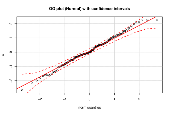
| Title produced by software | ML Fitting and QQ Plot- Normal Distribution | |||||||||||||||||||||||||||||||||||||||||||||||
| Date of computation | Thu, 04 Oct 2018 13:05:30 +0200 | |||||||||||||||||||||||||||||||||||||||||||||||
| Cite this page as follows | Statistical Computations at FreeStatistics.org, Office for Research Development and Education, URL https://freestatistics.org/blog/index.php?v=date/2018/Oct/04/t15386513209m9iyvh4jdtp8om.htm/, Retrieved Fri, 10 May 2024 09:25:58 +0000 | |||||||||||||||||||||||||||||||||||||||||||||||
| Statistical Computations at FreeStatistics.org, Office for Research Development and Education, URL https://freestatistics.org/blog/index.php?pk=315557, Retrieved Fri, 10 May 2024 09:25:58 +0000 | ||||||||||||||||||||||||||||||||||||||||||||||||
| QR Codes: | ||||||||||||||||||||||||||||||||||||||||||||||||
|
| ||||||||||||||||||||||||||||||||||||||||||||||||
| Original text written by user: | ||||||||||||||||||||||||||||||||||||||||||||||||
| IsPrivate? | No (this computation is public) | |||||||||||||||||||||||||||||||||||||||||||||||
| User-defined keywords | ||||||||||||||||||||||||||||||||||||||||||||||||
| Estimated Impact | 115 | |||||||||||||||||||||||||||||||||||||||||||||||
Tree of Dependent Computations | ||||||||||||||||||||||||||||||||||||||||||||||||
| Family? (F = Feedback message, R = changed R code, M = changed R Module, P = changed Parameters, D = changed Data) | ||||||||||||||||||||||||||||||||||||||||||||||||
| - [ML Fitting and QQ Plot- Normal Distribution] [] [2018-10-04 11:05:30] [fe87f86f8a649e8dd232440b9db78f3e] [Current] | ||||||||||||||||||||||||||||||||||||||||||||||||
| Feedback Forum | ||||||||||||||||||||||||||||||||||||||||||||||||
Post a new message | ||||||||||||||||||||||||||||||||||||||||||||||||
Dataset | ||||||||||||||||||||||||||||||||||||||||||||||||
| Dataseries X: | ||||||||||||||||||||||||||||||||||||||||||||||||
0.5204858765 0.4299970622 0.1055749243 0.8839177281 -0.2776217713 -0.04603036369 1.530298233 1.494731706 -0.02891792556 0.6210498591 -0.6833539359 -0.3082249829 2.280133308 -0.8854543504 -0.04417164204 -0.2627590147 -0.6464459948 -1.408271427 -0.2068236471 -0.2444683685 -0.5751587313 1.097042084 0.1405691781 -0.3300974353 0.1428316656 0.5221842551 0.4357357906 -0.3140161459 0.5044406113 -0.8869340522 -0.5515685025 0.3221753874 -0.1657235598 0.5236439193 0.5334899411 -0.01308235838 -0.188870343 -1.583371452 -0.06925025675 -0.8971631937 -0.4586626014 0.6110670481 2.111856211 0.7777655572 -0.3209775348 -0.2231985481 1.173938281 0.02263852571 0.5932077408 1.675801559 -0.719839903 0.5162627183 -0.4181946087 -0.04962701844 -0.8528521942 0.9169631383 2.132480975 -0.5417598275 1.579291362 -1.278896837 1.230393048 1.154504413 -0.9500787618 -0.3315198443 -0.287192948 0.5204767549 -2.670639646 -0.3054041115 0.6705847742 0.5393860559 0.1598504595 1.429802307 -0.1034513415 -0.7810377769 -1.022645695 0.2453215126 -1.619279166 -0.3391061191 0.6802321487 0.8461418237 -0.1475624525 0.6771614217 -0.5552064271 -1.589212028 0.3693384673 0.9532453187 0.5877242327 1.277966617 -0.0467692114 0.7582087478 -1.524612327 -0.8199127865 -0.7271715052 1.201655844 -0.519997947 0.02365677181 -0.6266331882 0.03756465409 -0.01730812214 -0.7834487515 0.4530912767 -1.985004931 -1.57658523 0.5421603989 0.6866220024 -0.2243281006 -0.6022367528 -1.419591408 1.095193078 1.298443003 1.800641426 -1.324349799 1.463766685 -0.1093880669 1.016816844 -0.5485597733 0.3050223862 0.7261463821 0.1583472137 -0.1278204388 -2.129778564 -1.069239212 0.3488821306 -0.148364031 -1.793054034 0.2138747947 1.054839856 0.4083389505 2.263713378 1.047445731 0.4634591175 0.3678508639 -0.9585346633 0.3916771173 -0.09227420385 -0.3880879866 -0.20806761 1.967601235 -1.661825274 -0.125538702 2.262872815 1.076537534 -0.1584336002 0.08453179444 -1.00981273 0.9664253567 1.206438862 1.256021171 -1.363092143 1.745031988 | ||||||||||||||||||||||||||||||||||||||||||||||||
Tables (Output of Computation) | ||||||||||||||||||||||||||||||||||||||||||||||||
| ||||||||||||||||||||||||||||||||||||||||||||||||
Figures (Output of Computation) | ||||||||||||||||||||||||||||||||||||||||||||||||
Input Parameters & R Code | ||||||||||||||||||||||||||||||||||||||||||||||||
| Parameters (Session): | ||||||||||||||||||||||||||||||||||||||||||||||||
| par1 = 8 ; par2 = 0 ; | ||||||||||||||||||||||||||||||||||||||||||||||||
| Parameters (R input): | ||||||||||||||||||||||||||||||||||||||||||||||||
| par1 = 8 ; par2 = 0 ; | ||||||||||||||||||||||||||||||||||||||||||||||||
| R code (references can be found in the software module): | ||||||||||||||||||||||||||||||||||||||||||||||||
library(MASS) | ||||||||||||||||||||||||||||||||||||||||||||||||