Free Statistics

of Irreproducible Research!

Author's title

Author*Unverified author*
R Software Modulerwasp_cross.wasp
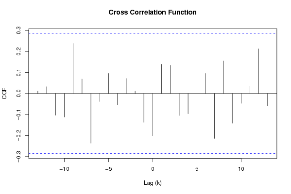
Title produced by softwareCross Correlation Function
Date of computationTue, 02 Dec 2008 04:13:28 -0700
Cite this page as followsStatistical Computations at FreeStatistics.org, Office for Research Development and Education, URL https://freestatistics.org/blog/index.php?v=date/2008/Dec/02/t1228216456qeqo20ddkcub0y1.htm/, Retrieved Tue, 27 Oct 2026 15:45:10 +0000
Statistical Computations at FreeStatistics.org, Office for Research Development and Education, URL https://freestatistics.org/blog/index.php?pk=27603, Retrieved Tue, 27 Oct 2026 15:45:10 +0000
QR Codes:

Original text written by user:
IsPrivate?No (this computation is public)
User-defined keywords
Estimated Impact576
Family? (F = Feedback message, R = changed R code, M = changed R Module, P = changed Parameters, D = changed Data)
F     [Law of Averages] [Random Walk Simul...] [2008-11-25 18:31:28] [b98453cac15ba1066b407e146608df68]
F RMPD    [Cross Correlation Function] [Workshop 4] [2008-12-02 11:13:28] [34b2bf1c29318ebc3536134756a32b87] [Current]
Feedback Forum
2008-12-06 19:18:13 [Stefan Temmerman] [reply] 
De student heeft de analyse goed uitgevoerd om de tijdreeks stationair te maken. Geen enkele correlatie bevindt zich nog boven het betrouwheidsinterval, en dus voorspelt X(t) niet meer Y(t).
2008-12-08 20:06:15 [An Knapen] [reply] 
Bij deze vraag heeft de student duidelijk vermeld welke waarden de parameters hebben. lambda =1 d=1 en D=1
We kunnen duidelijk zien dat de correlatie positief als negatief kan zijn. De staafjes liggen nu echter wel binnen het betrouwbaarheidsinterval. Dit resultaat heeft men bekomen door seizoenaal en niet-seizoenaal te differentiëren. De lange termijn trend en de seizoenaliteit zijn volledig verdwenen

Post a new message
Dataseries X:
87.0
96.3
107.1
115.2
106.1
89.5
91.3
97.6
100.7
104.6
94.7
101.8
102.5
105.3
110.3
109.8
117.3
118.8
131.3
125.9
133.1
147.0
145.8
164.4
149.8
137.7
151.7
156.8
180.0
180.4
170.4
191.6
199.5
218.2
217.5
205.0
194.0
199.3
219.3
211.1
215.2
240.2
242.2
240.7
255.4
253.0
218.2
203.7
205.6
215.6
188.5
202.9
214.0
230.3
230.0
241.0
259.6
247.8
270.3
289.7
Dataseries Y:
106.7
101.1
97.8
113.8
107.1
117.5
113.7
106.6
109.8
108.8
102.0
114.5
116.5
108.6
113.9
109.3
112.5
123.4
115.2
110.8
120.4
117.6
111.2
131.1
118.9
115.7
119.6
113.1
106.4
115.5
111.8
109.6
121.5
109.5
109.0
113.4
112.7
114.4
109.2
116.2
113.8
123.6
112.6
117.7
113.3
110.7
114.7
116.9
120.6
111.6
111.9
116.1
111.9
125.1
115.1
116.7
115.8
116.8
113.0
106.5


Summary of computational transaction
Raw Inputview raw input (R code)
Raw Outputview raw output of R engine
Computing time1 seconds
R Server'Gwilym Jenkins' @ 72.249.127.135

\begin{tabular}{lllllllll}
\hline
Summary of computational transaction \tabularnewline
Raw Input & view raw input (R code)  \tabularnewline
Raw Output & view raw output of R engine  \tabularnewline
Computing time & 1 seconds \tabularnewline
R Server & 'Gwilym Jenkins' @ 72.249.127.135 \tabularnewline
\hline
\end{tabular}
%Source: https://freestatistics.org/blog/index.php?pk=27603&T=0

[TABLE]
[ROW][C]Summary of computational transaction[/C][/ROW]
[ROW][C]Raw Input[/C][C]view raw input (R code) [/C][/ROW]
[ROW][C]Raw Output[/C][C]view raw output of R engine [/C][/ROW]
[ROW][C]Computing time[/C][C]1 seconds[/C][/ROW]
[ROW][C]R Server[/C][C]'Gwilym Jenkins' @ 72.249.127.135[/C][/ROW]
[/TABLE]
Source: https://freestatistics.org/blog/index.php?pk=27603&T=0

Globally Unique Identifier (entire table): ba.freestatistics.org/blog/index.php?pk=27603&T=0

As an alternative you can also use a QR Code:  

The GUIDs for individual cells are displayed in the table below:

Summary of computational transaction
Raw Inputview raw input (R code)
Raw Outputview raw output of R engine
Computing time1 seconds
R Server'Gwilym Jenkins' @ 72.249.127.135


Cross Correlation Function
ParameterValue
Box-Cox transformation parameter (lambda) of X series1
Degree of non-seasonal differencing (d) of X series1
Degree of seasonal differencing (D) of X series1
Seasonal Period (s)12
Box-Cox transformation parameter (lambda) of Y series1
Degree of non-seasonal differencing (d) of Y series1
Degree of seasonal differencing (D) of Y series1
krho(Y[t],X[t+k])
-130.0115773515609963
-120.0326307264809896
-11-0.103695699644002
-10-0.112176822713199
-90.238404019107931
-80.0689235520610102
-7-0.236212198281189
-6-0.0381334364921076
-50.0955768711877626
-4-0.05331431975496
-30.0718477408493209
-20.0111436222256402
-1-0.136974556861736
0-0.200434422235479
10.139252429951621
20.134330143265683
3-0.104629309979149
4-0.0963682278946863
50.0306331147543409
60.0956149545810556
7-0.21397512667486
80.15517978013441
9-0.141426359686365
10-0.0467547712714196
110.0354401789184439
120.212639226060947
13-0.059430285837986

\begin{tabular}{lllllllll}
\hline
Cross Correlation Function \tabularnewline
Parameter & Value \tabularnewline
Box-Cox transformation parameter (lambda) of X series & 1 \tabularnewline
Degree of non-seasonal differencing (d) of X series & 1 \tabularnewline
Degree of seasonal differencing (D) of X series & 1 \tabularnewline
Seasonal Period (s) & 12 \tabularnewline
Box-Cox transformation parameter (lambda) of Y series & 1 \tabularnewline
Degree of non-seasonal differencing (d) of Y series & 1 \tabularnewline
Degree of seasonal differencing (D) of Y series & 1 \tabularnewline
k & rho(Y[t],X[t+k]) \tabularnewline
-13 & 0.0115773515609963 \tabularnewline
-12 & 0.0326307264809896 \tabularnewline
-11 & -0.103695699644002 \tabularnewline
-10 & -0.112176822713199 \tabularnewline
-9 & 0.238404019107931 \tabularnewline
-8 & 0.0689235520610102 \tabularnewline
-7 & -0.236212198281189 \tabularnewline
-6 & -0.0381334364921076 \tabularnewline
-5 & 0.0955768711877626 \tabularnewline
-4 & -0.05331431975496 \tabularnewline
-3 & 0.0718477408493209 \tabularnewline
-2 & 0.0111436222256402 \tabularnewline
-1 & -0.136974556861736 \tabularnewline
0 & -0.200434422235479 \tabularnewline
1 & 0.139252429951621 \tabularnewline
2 & 0.134330143265683 \tabularnewline
3 & -0.104629309979149 \tabularnewline
4 & -0.0963682278946863 \tabularnewline
5 & 0.0306331147543409 \tabularnewline
6 & 0.0956149545810556 \tabularnewline
7 & -0.21397512667486 \tabularnewline
8 & 0.15517978013441 \tabularnewline
9 & -0.141426359686365 \tabularnewline
10 & -0.0467547712714196 \tabularnewline
11 & 0.0354401789184439 \tabularnewline
12 & 0.212639226060947 \tabularnewline
13 & -0.059430285837986 \tabularnewline
\hline
\end{tabular}
%Source: https://freestatistics.org/blog/index.php?pk=27603&T=1

[TABLE]
[ROW][C]Cross Correlation Function[/C][/ROW]
[ROW][C]Parameter[/C][C]Value[/C][/ROW]
[ROW][C]Box-Cox transformation parameter (lambda) of X series[/C][C]1[/C][/ROW]
[ROW][C]Degree of non-seasonal differencing (d) of X series[/C][C]1[/C][/ROW]
[ROW][C]Degree of seasonal differencing (D) of X series[/C][C]1[/C][/ROW]
[ROW][C]Seasonal Period (s)[/C][C]12[/C][/ROW]
[ROW][C]Box-Cox transformation parameter (lambda) of Y series[/C][C]1[/C][/ROW]
[ROW][C]Degree of non-seasonal differencing (d) of Y series[/C][C]1[/C][/ROW]
[ROW][C]Degree of seasonal differencing (D) of Y series[/C][C]1[/C][/ROW]
[ROW][C]k[/C][C]rho(Y[t],X[t+k])[/C][/ROW]
[ROW][C]-13[/C][C]0.0115773515609963[/C][/ROW]
[ROW][C]-12[/C][C]0.0326307264809896[/C][/ROW]
[ROW][C]-11[/C][C]-0.103695699644002[/C][/ROW]
[ROW][C]-10[/C][C]-0.112176822713199[/C][/ROW]
[ROW][C]-9[/C][C]0.238404019107931[/C][/ROW]
[ROW][C]-8[/C][C]0.0689235520610102[/C][/ROW]
[ROW][C]-7[/C][C]-0.236212198281189[/C][/ROW]
[ROW][C]-6[/C][C]-0.0381334364921076[/C][/ROW]
[ROW][C]-5[/C][C]0.0955768711877626[/C][/ROW]
[ROW][C]-4[/C][C]-0.05331431975496[/C][/ROW]
[ROW][C]-3[/C][C]0.0718477408493209[/C][/ROW]
[ROW][C]-2[/C][C]0.0111436222256402[/C][/ROW]
[ROW][C]-1[/C][C]-0.136974556861736[/C][/ROW]
[ROW][C]0[/C][C]-0.200434422235479[/C][/ROW]
[ROW][C]1[/C][C]0.139252429951621[/C][/ROW]
[ROW][C]2[/C][C]0.134330143265683[/C][/ROW]
[ROW][C]3[/C][C]-0.104629309979149[/C][/ROW]
[ROW][C]4[/C][C]-0.0963682278946863[/C][/ROW]
[ROW][C]5[/C][C]0.0306331147543409[/C][/ROW]
[ROW][C]6[/C][C]0.0956149545810556[/C][/ROW]
[ROW][C]7[/C][C]-0.21397512667486[/C][/ROW]
[ROW][C]8[/C][C]0.15517978013441[/C][/ROW]
[ROW][C]9[/C][C]-0.141426359686365[/C][/ROW]
[ROW][C]10[/C][C]-0.0467547712714196[/C][/ROW]
[ROW][C]11[/C][C]0.0354401789184439[/C][/ROW]
[ROW][C]12[/C][C]0.212639226060947[/C][/ROW]
[ROW][C]13[/C][C]-0.059430285837986[/C][/ROW]
[/TABLE]
Source: https://freestatistics.org/blog/index.php?pk=27603&T=1

Globally Unique Identifier (entire table): ba.freestatistics.org/blog/index.php?pk=27603&T=1

As an alternative you can also use a QR Code:  

The GUIDs for individual cells are displayed in the table below:

Cross Correlation Function
ParameterValue
Box-Cox transformation parameter (lambda) of X series1
Degree of non-seasonal differencing (d) of X series1
Degree of seasonal differencing (D) of X series1
Seasonal Period (s)12
Box-Cox transformation parameter (lambda) of Y series1
Degree of non-seasonal differencing (d) of Y series1
Degree of seasonal differencing (D) of Y series1
krho(Y[t],X[t+k])
-130.0115773515609963
-120.0326307264809896
-11-0.103695699644002
-10-0.112176822713199
-90.238404019107931
-80.0689235520610102
-7-0.236212198281189
-6-0.0381334364921076
-50.0955768711877626
-4-0.05331431975496
-30.0718477408493209
-20.0111436222256402
-1-0.136974556861736
0-0.200434422235479
10.139252429951621
20.134330143265683
3-0.104629309979149
4-0.0963682278946863
50.0306331147543409
60.0956149545810556
7-0.21397512667486
80.15517978013441
9-0.141426359686365
10-0.0467547712714196
110.0354401789184439
120.212639226060947
13-0.059430285837986


Parameters (Session):
par1 = 1 ; par2 = 1 ; par3 = 1 ; par4 = 12 ; par5 = 1 ; par6 = 1 ; par7 = 1 ;
Parameters (R input):
par1 = 1 ; par2 = 1 ; par3 = 1 ; par4 = 12 ; par5 = 1 ; par6 = 1 ; par7 = 1 ;
R code (references can be found in the software module):
par1 <- as.numeric(par1)
par2 <- as.numeric(par2)
par3 <- as.numeric(par3)
par4 <- as.numeric(par4)
par5 <- as.numeric(par5)
par6 <- as.numeric(par6)
par7 <- as.numeric(par7)
if (par1 == 0) {
x <- log(x)
} else {
x <- (x ^ par1 - 1) / par1
}
if (par5 == 0) {
y <- log(y)
} else {
y <- (y ^ par5 - 1) / par5
}
if (par2 > 0) x <- diff(x,lag=1,difference=par2)
if (par6 > 0) y <- diff(y,lag=1,difference=par6)
if (par3 > 0) x <- diff(x,lag=par4,difference=par3)
if (par7 > 0) y <- diff(y,lag=par4,difference=par7)
x
y
bitmap(file='test1.png')
(r <- ccf(x,y,main='Cross Correlation Function',ylab='CCF',xlab='Lag (k)'))
dev.off()
load(file='createtable')
a<-table.start()
a<-table.row.start(a)
a<-table.element(a,'Cross Correlation Function',2,TRUE)
a<-table.row.end(a)
a<-table.row.start(a)
a<-table.element(a,'Parameter',header=TRUE)
a<-table.element(a,'Value',header=TRUE)
a<-table.row.end(a)
a<-table.row.start(a)
a<-table.element(a,'Box-Cox transformation parameter (lambda) of X series',header=TRUE)
a<-table.element(a,par1)
a<-table.row.end(a)
a<-table.row.start(a)
a<-table.element(a,'Degree of non-seasonal differencing (d) of X series',header=TRUE)
a<-table.element(a,par2)
a<-table.row.end(a)
a<-table.row.start(a)
a<-table.element(a,'Degree of seasonal differencing (D) of X series',header=TRUE)
a<-table.element(a,par3)
a<-table.row.end(a)
a<-table.row.start(a)
a<-table.element(a,'Seasonal Period (s)',header=TRUE)
a<-table.element(a,par4)
a<-table.row.end(a)
a<-table.row.start(a)
a<-table.element(a,'Box-Cox transformation parameter (lambda) of Y series',header=TRUE)
a<-table.element(a,par5)
a<-table.row.end(a)
a<-table.row.start(a)
a<-table.element(a,'Degree of non-seasonal differencing (d) of Y series',header=TRUE)
a<-table.element(a,par6)
a<-table.row.end(a)
a<-table.row.start(a)
a<-table.element(a,'Degree of seasonal differencing (D) of Y series',header=TRUE)
a<-table.element(a,par7)
a<-table.row.end(a)
a<-table.row.start(a)
a<-table.element(a,'k',header=TRUE)
a<-table.element(a,'rho(Y[t],X[t+k])',header=TRUE)
a<-table.row.end(a)
mylength <- length(r$acf)
myhalf <- floor((mylength-1)/2)
for (i in 1:mylength) {
a<-table.row.start(a)
a<-table.element(a,i-myhalf-1,header=TRUE)
a<-table.element(a,r$acf[i])
a<-table.row.end(a)
}
a<-table.end(a)
table.save(a,file='mytable.tab')