Free Statistics

of Irreproducible Research!

Author's title

Author*The author of this computation has been verified*
R Software Modulerwasp_meanplot.wasp
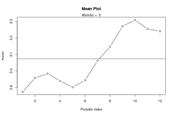
Title produced by softwareMean Plot
Date of computationMon, 03 Nov 2008 11:06:22 -0700
Cite this page as followsStatistical Computations at FreeStatistics.org, Office for Research Development and Education, URL https://freestatistics.org/blog/index.php?v=date/2008/Nov/03/t12257357149trif7rdarbm1no.htm/, Retrieved Tue, 29 Sep 2026 08:15:51 +0000
Statistical Computations at FreeStatistics.org, Office for Research Development and Education, URL https://freestatistics.org/blog/index.php?pk=20924, Retrieved Tue, 29 Sep 2026 08:15:51 +0000
QR Codes:

Original text written by user:
IsPrivate?No (this computation is public)
User-defined keywords
Estimated Impact456
Family? (F = Feedback message, R = changed R code, M = changed R Module, P = changed Parameters, D = changed Data)
F       [Mean Plot] [Hypothesis Testin...] [2008-11-03 18:06:22] [c33ddd06d9ea3933c8ac89c0e74c9b3a] [Current]
Feedback Forum
2008-11-07 15:01:03 [Jeroen Aerts] [reply] 
Ik vermoed dat hier geen seizoensgebondenheid is.

Eerst en vooral kijk ik naar eigen logica. Het lijkt me niet logisch dat de deze rentevoet van de schatkistcertificaten seizoensgebonden kan zijn. ( Waarom zou een stijging/daling van de rentevoet schatkistcertificaten immers afhankelijk kunnen zijn van de seizoenen?)

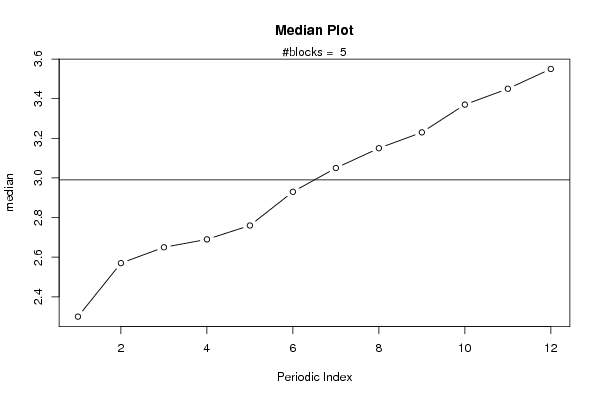
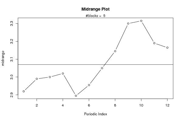
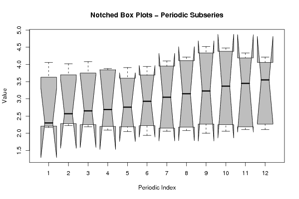
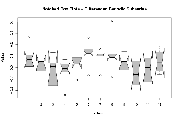
En als je kijkt naar de Notched box plots - periodic subseries zie je dat, welke maanden je ook vergelijkt, de betrouwbaarheidsintervallen ongeveer gelijk zijn, daaruit kan je concluderen dat een stijging/daling van het gemiddelde eerder een 'toevalligheid' kan genoemd worden en géén 'significant' verschil.

Post a new message
Dataseries X:
2.17
2.28
2.25
2.09
2.05
1.94
2.06
2.18
2.27
2.25
2.19
2.27
2.21
2.22
2.19
2.2
2.19
2.22
2.15
2.08
2
2.06
2.11
2.11
2.3
2.57
2.65
2.69
2.76
2.93
3.05
3.15
3.23
3.37
3.45
3.55
3.63
3.7
3.75
3.88
3.91
3.94
4.1
4.21
4.33
4.38
4.19
4.06
4.06
4.02
4.08
3.84
3.6
3.69
3.95
4.11
4.52
4.48
4.33
4.21


Summary of computational transaction
Raw Inputview raw input (R code)
Raw Outputview raw output of R engine
Computing time4 seconds
R Server'Herman Ole Andreas Wold' @ 193.190.124.10:1001

\begin{tabular}{lllllllll}
\hline
Summary of computational transaction \tabularnewline
Raw Input & view raw input (R code)  \tabularnewline
Raw Output & view raw output of R engine  \tabularnewline
Computing time & 4 seconds \tabularnewline
R Server & 'Herman Ole Andreas Wold' @ 193.190.124.10:1001 \tabularnewline
\hline
\end{tabular}
%Source: https://freestatistics.org/blog/index.php?pk=20924&T=0

[TABLE]
[ROW][C]Summary of computational transaction[/C][/ROW]
[ROW][C]Raw Input[/C][C]view raw input (R code) [/C][/ROW]
[ROW][C]Raw Output[/C][C]view raw output of R engine [/C][/ROW]
[ROW][C]Computing time[/C][C]4 seconds[/C][/ROW]
[ROW][C]R Server[/C][C]'Herman Ole Andreas Wold' @ 193.190.124.10:1001[/C][/ROW]
[/TABLE]
Source: https://freestatistics.org/blog/index.php?pk=20924&T=0

Globally Unique Identifier (entire table): ba.freestatistics.org/blog/index.php?pk=20924&T=0

As an alternative you can also use a QR Code:  

The GUIDs for individual cells are displayed in the table below:

Summary of computational transaction
Raw Inputview raw input (R code)
Raw Outputview raw output of R engine
Computing time4 seconds
R Server'Herman Ole Andreas Wold' @ 193.190.124.10:1001


Parameters (Session):
par1 = 12 ;
Parameters (R input):
par1 = 12 ;
R code (references can be found in the software module):
par1 <- as.numeric(par1)
(n <- length(x))
(np <- floor(n / par1))
arr <- array(NA,dim=c(par1,np+1))
darr <- array(NA,dim=c(par1,np+1))
ari <- array(0,dim=par1)
dx <- diff(x)
j <- 0
for (i in 1:n)
{
j = j + 1
ari[j] = ari[j] + 1
arr[j,ari[j]] <- x[i]
darr[j,ari[j]] <- dx[i]
if (j == par1) j = 0
}
ari
arr
darr
arr.mean <- array(NA,dim=par1)
arr.median <- array(NA,dim=par1)
arr.midrange <- array(NA,dim=par1)
for (j in 1:par1)
{
arr.mean[j] <- mean(arr[j,],na.rm=TRUE)
arr.median[j] <- median(arr[j,],na.rm=TRUE)
arr.midrange[j] <- (quantile(arr[j,],0.75,na.rm=TRUE) + quantile(arr[j,],0.25,na.rm=TRUE)) / 2
}
overall.mean <- mean(x)
overall.median <- median(x)
overall.midrange <- (quantile(x,0.75) + quantile(x,0.25)) / 2
bitmap(file='plot1.png')
plot(arr.mean,type='b',ylab='mean',main='Mean Plot',xlab='Periodic Index')
mtext(paste('#blocks = ',np))
abline(overall.mean,0)
dev.off()
bitmap(file='plot2.png')
plot(arr.median,type='b',ylab='median',main='Median Plot',xlab='Periodic Index')
mtext(paste('#blocks = ',np))
abline(overall.median,0)
dev.off()
bitmap(file='plot3.png')
plot(arr.midrange,type='b',ylab='midrange',main='Midrange Plot',xlab='Periodic Index')
mtext(paste('#blocks = ',np))
abline(overall.midrange,0)
dev.off()
bitmap(file='plot4.png')
z <- data.frame(t(arr))
names(z) <- c(1:par1)
(boxplot(z,notch=TRUE,col='grey',xlab='Periodic Index',ylab='Value',main='Notched Box Plots - Periodic Subseries'))
dev.off()
bitmap(file='plot4b.png')
z <- data.frame(t(darr))
names(z) <- c(1:par1)
(boxplot(z,notch=TRUE,col='grey',xlab='Periodic Index',ylab='Value',main='Notched Box Plots - Differenced Periodic Subseries'))
dev.off()
bitmap(file='plot5.png')
z <- data.frame(arr)
names(z) <- c(1:np)
(boxplot(z,notch=TRUE,col='grey',xlab='Block Index',ylab='Value',main='Notched Box Plots - Sequential Blocks'))
dev.off()
bitmap(file='plot6.png')
z <- data.frame(cbind(arr.mean,arr.median,arr.midrange))
names(z) <- list('mean','median','midrange')
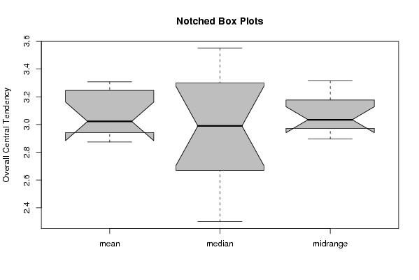
(boxplot(z,notch=TRUE,col='grey',ylab='Overall Central Tendency',main='Notched Box Plots'))
dev.off()