Free Statistics
of Irreproducible Research!
Description of Statistical Computation | |||||||||||||||||||||||||||||||||||||||||||||||||
|---|---|---|---|---|---|---|---|---|---|---|---|---|---|---|---|---|---|---|---|---|---|---|---|---|---|---|---|---|---|---|---|---|---|---|---|---|---|---|---|---|---|---|---|---|---|---|---|---|---|
| Author's title | |||||||||||||||||||||||||||||||||||||||||||||||||
| Author | *The author of this computation has been verified* | ||||||||||||||||||||||||||||||||||||||||||||||||
| R Software Module | rwasp_tukeylambda.wasp | ||||||||||||||||||||||||||||||||||||||||||||||||
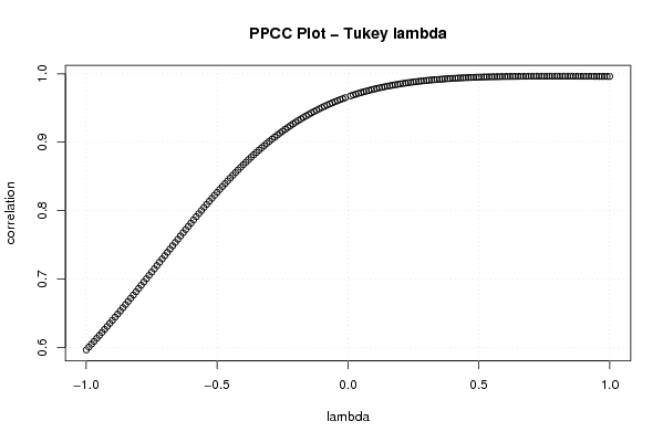
| Title produced by software | Tukey lambda PPCC Plot | ||||||||||||||||||||||||||||||||||||||||||||||||
| Date of computation | Fri, 24 Oct 2008 11:27:20 -0600 | ||||||||||||||||||||||||||||||||||||||||||||||||
| Cite this page as follows | Statistical Computations at FreeStatistics.org, Office for Research Development and Education, URL https://freestatistics.org/blog/index.php?v=date/2008/Oct/24/t1224869309cva6cnqpd8lr8c8.htm/, Retrieved Sun, 25 Oct 2026 08:30:35 +0000 | ||||||||||||||||||||||||||||||||||||||||||||||||
| Statistical Computations at FreeStatistics.org, Office for Research Development and Education, URL https://freestatistics.org/blog/index.php?pk=18656, Retrieved Sun, 25 Oct 2026 08:30:35 +0000 | |||||||||||||||||||||||||||||||||||||||||||||||||
| QR Codes: | |||||||||||||||||||||||||||||||||||||||||||||||||
|
| |||||||||||||||||||||||||||||||||||||||||||||||||
| Original text written by user: | |||||||||||||||||||||||||||||||||||||||||||||||||
| IsPrivate? | No (this computation is public) | ||||||||||||||||||||||||||||||||||||||||||||||||
| User-defined keywords | |||||||||||||||||||||||||||||||||||||||||||||||||
| Estimated Impact | 537 | ||||||||||||||||||||||||||||||||||||||||||||||||
Tree of Dependent Computations | |||||||||||||||||||||||||||||||||||||||||||||||||
| Family? (F = Feedback message, R = changed R code, M = changed R Module, P = changed Parameters, D = changed Data) | |||||||||||||||||||||||||||||||||||||||||||||||||
| F [Tukey lambda PPCC Plot] [Investigating Dis...] [2007-10-21 16:01:20] [b9964c45117f7aac638ab9056d451faa] F D [Tukey lambda PPCC Plot] [Associating Distr...] [2008-10-24 16:19:53] [a57f5cc542637534b8bb5bcb4d37eab1] F D [Tukey lambda PPCC Plot] [Investigating Dis...] [2008-10-24 17:27:20] [0f30549460cf4ec26d9cf94b1fcf7789] [Current] | |||||||||||||||||||||||||||||||||||||||||||||||||
| Feedback Forum | |||||||||||||||||||||||||||||||||||||||||||||||||
Post a new message | |||||||||||||||||||||||||||||||||||||||||||||||||
Dataset | |||||||||||||||||||||||||||||||||||||||||||||||||
| Dataseries X: | |||||||||||||||||||||||||||||||||||||||||||||||||
106,60 106,80 107,00 107,10 107,30 107,40 107,60 107,70 107,90 108,20 108,30 108,50 108,92 109,23 109,41 109,65 109,91 110,01 110,20 110,49 110,57 110,72 110,94 111,09 111,28 111,41 111,62 111,76 111,89 112,04 112,12 112,30 112,47 112,59 112,78 112,73 112,99 113,10 113,33 113,38 113,68 113,65 113,81 113,88 114,02 114,25 114,28 114,38 114,73 114,97 115,05 115,29 115,37 115,54 115,76 115,92 116,02 116,21 116,26 116,51 | |||||||||||||||||||||||||||||||||||||||||||||||||
Tables (Output of Computation) | |||||||||||||||||||||||||||||||||||||||||||||||||
| |||||||||||||||||||||||||||||||||||||||||||||||||
Figures (Output of Computation) | |||||||||||||||||||||||||||||||||||||||||||||||||
Input Parameters & R Code | |||||||||||||||||||||||||||||||||||||||||||||||||
| Parameters (Session): | |||||||||||||||||||||||||||||||||||||||||||||||||
| Parameters (R input): | |||||||||||||||||||||||||||||||||||||||||||||||||
| R code (references can be found in the software module): | |||||||||||||||||||||||||||||||||||||||||||||||||
gp <- function(lambda, p) | |||||||||||||||||||||||||||||||||||||||||||||||||