Repository of Reproducible Computations

Free Statistics

of Irreproducible Research!

Author's title

Author

*The author of this computation has been verified*

R Software Module

rwasp_arimaforecasting.wasp

Title produced by software

ARIMA Forecasting

Date of computation

Wed, 09 Dec 2009 09:48:03 -0700

Cite this page as follows

Statistical Computations at FreeStatistics.org, Office for Research Development and Education, URL https://freestatistics.org/blog/index.php?v=date/2009/Dec/09/t1260377576i5x2uqzx5gbhefe.htm/, Retrieved Sat, 27 Apr 2024 06:01:45 +0000

Statistical Computations at FreeStatistics.org, Office for Research Development and Education, URL https://freestatistics.org/blog/index.php?pk=65046, Retrieved Sat, 27 Apr 2024 06:01:45 +0000

QR Codes:

Paste this QR Code to cite your computation.

Original text written by user:

IsPrivate?

No (this computation is public)

User-defined keywords

Estimated Impact

181

Family? (F = Feedback message, R = changed R code, M = changed R Module, P = changed Parameters, D = changed Data)

-     [ARIMA Forecasting] [] [2009-12-07 09:54:52] [b98453cac15ba1066b407e146608df68]
- R PD    [ARIMA Forecasting] [ARIMA-Forecasting] [2009-12-09 16:48:03] [acc980be4047884b6edd254cd7beb9fa] [Current]
-   PD      [ARIMA Forecasting] [ARIMA forecasting] [2009-12-10 08:34:29] [a542c511726eba04a1fc2f4bd37a90f8] 
-   P         [ARIMA Forecasting] [] [2009-12-10 10:17:58] [a542c511726eba04a1fc2f4bd37a90f8] 
-   PD        [ARIMA Forecasting] [Arima forecasting] [2009-12-11 20:47:14] [76ab39dc7a55316678260825bd5ad46c] 
-   PD          [ARIMA Forecasting] [ARIMA forecasting] [2009-12-11 22:18:44] [4b453aa14d54730625f8d3de5f1f6d82] 
-           [ARIMA Forecasting] [] [2009-12-11 12:33:06] [1c9e2d56abd8ff474f03ef7df8c5b4d9] 
-   PD      [ARIMA Forecasting] [] [2009-12-11 14:14:48] [1c9e2d56abd8ff474f03ef7df8c5b4d9] 
-   PD      [ARIMA Forecasting] [Forecast] [2009-12-20 12:55:02] [36becc366f59efff5c3495030cea7527] 

Feedback Forum

Post a new message

Dataseries X:

Download CSV

Histogram

Boxplots

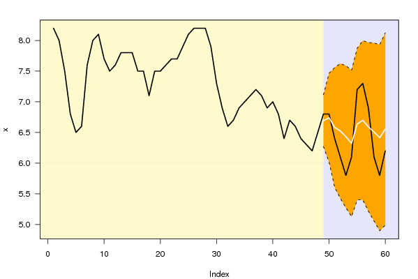
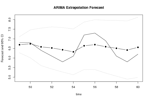
8.2
8
7.5
6.8
6.5
6.6
7.6
8
8.1
7.7
7.5
7.6
7.8
7.8
7.8
7.5
7.5
7.1
7.5
7.5
7.6
7.7
7.7
7.9
8.1
8.2
8.2
8.2
7.9
7.3
6.9
6.6
6.7
6.9
7
7.1
7.2
7.1
6.9
7
6.8
6.4
6.7
6.6
6.4
6.3
6.2
6.5
6.8
6.8
6.4
6.1
5.8
6.1
7.2
7.3
6.9
6.1
5.8
6.2

Summary of computational transaction
Raw Input	view raw input (R code)
Raw Output	view raw output of R engine
Computing time	4 seconds
R Server	'Gwilym Jenkins' @ 72.249.127.135

\begin{tabular}{lllllllll}
\hline
Summary of computational transaction \tabularnewline
Raw Input & view raw input (R code)  \tabularnewline
Raw Output & view raw output of R engine  \tabularnewline
Computing time & 4 seconds \tabularnewline
R Server & 'Gwilym Jenkins' @ 72.249.127.135 \tabularnewline
\hline
\end{tabular}
%Source: https://freestatistics.org/blog/index.php?pk=65046&T=0

[TABLE]
[ROW][C]Summary of computational transaction[/C][/ROW]
[ROW][C]Raw Input[/C][C]view raw input (R code) [/C][/ROW]
[ROW][C]Raw Output[/C][C]view raw output of R engine [/C][/ROW]
[ROW][C]Computing time[/C][C]4 seconds[/C][/ROW]
[ROW][C]R Server[/C][C]'Gwilym Jenkins' @ 72.249.127.135[/C][/ROW]
[/TABLE]
Source: https://freestatistics.org/blog/index.php?pk=65046&T=0

Globally Unique Identifier (entire table): ba.freestatistics.org/blog/index.php?pk=65046&T=0

As an alternative you can also use a QR Code:

The GUIDs for individual cells are displayed in the table below:

Summary of computational transaction
Raw Input	view raw input (R code)
Raw Output	view raw output of R engine
Computing time	4 seconds
R Server	'Gwilym Jenkins' @ 72.249.127.135

Univariate ARIMA Extrapolation Forecast
time	Y[t]	F[t]	95% LB	95% UB	p-value(H0: Y[t] = F[t])	P(F[t]>Y[t-1])	P(F[t]>Y[t-s])	P(F[t]>Y[48])
36	7.1	-	-	-	-	-	-	-
37	7.2	-	-	-	-	-	-	-
38	7.1	-	-	-	-	-	-	-
39	6.9	-	-	-	-	-	-	-
40	7	-	-	-	-	-	-	-
41	6.8	-	-	-	-	-	-	-
42	6.4	-	-	-	-	-	-	-
43	6.7	-	-	-	-	-	-	-
44	6.6	-	-	-	-	-	-	-
45	6.4	-	-	-	-	-	-	-
46	6.3	-	-	-	-	-	-	-
47	6.2	-	-	-	-	-	-	-
48	6.5	-	-	-	-	-	-	-
49	6.8	6.6922	6.2706	7.1139	0.3082	0.8142	0.0091	0.8142
50	6.8	6.7403	6.0139	7.4667	0.436	0.436	0.1659	0.7416
51	6.4	6.5815	5.6043	7.5588	0.3579	0.3306	0.2615	0.5649
52	6.1	6.5248	5.4265	7.6231	0.2242	0.5881	0.1982	0.5177
53	5.8	6.4296	5.2715	7.5877	0.1433	0.7115	0.2654	0.4526
54	6.1	6.3218	5.1279	7.5156	0.3579	0.8042	0.4489	0.3849
55	7.2	6.637	5.3999	7.8741	0.1862	0.8026	0.4602	0.5859
56	7.3	6.6979	5.3992	7.9966	0.1817	0.2243	0.5587	0.6174
57	6.9	6.5907	5.2145	7.9668	0.3298	0.1562	0.607	0.5514
58	6.1	6.5075	5.0553	7.9597	0.2912	0.2981	0.6103	0.504
59	5.8	6.4146	4.8982	7.9311	0.2135	0.6579	0.6093	0.4561
60	6.2	6.5567	4.9881	8.1253	0.3279	0.8278	0.5282	0.5282

\begin{tabular}{lllllllll}
\hline
Univariate ARIMA Extrapolation Forecast \tabularnewline
time & Y[t] & F[t] & 95% LB & 95% UB & p-value(H0: Y[t] = F[t]) & P(F[t]>Y[t-1]) & P(F[t]>Y[t-s]) & P(F[t]>Y[48]) \tabularnewline
36 & 7.1 & - & - & - & - & - & - & - \tabularnewline
37 & 7.2 & - & - & - & - & - & - & - \tabularnewline
38 & 7.1 & - & - & - & - & - & - & - \tabularnewline
39 & 6.9 & - & - & - & - & - & - & - \tabularnewline
40 & 7 & - & - & - & - & - & - & - \tabularnewline
41 & 6.8 & - & - & - & - & - & - & - \tabularnewline
42 & 6.4 & - & - & - & - & - & - & - \tabularnewline
43 & 6.7 & - & - & - & - & - & - & - \tabularnewline
44 & 6.6 & - & - & - & - & - & - & - \tabularnewline
45 & 6.4 & - & - & - & - & - & - & - \tabularnewline
46 & 6.3 & - & - & - & - & - & - & - \tabularnewline
47 & 6.2 & - & - & - & - & - & - & - \tabularnewline
48 & 6.5 & - & - & - & - & - & - & - \tabularnewline
49 & 6.8 & 6.6922 & 6.2706 & 7.1139 & 0.3082 & 0.8142 & 0.0091 & 0.8142 \tabularnewline
50 & 6.8 & 6.7403 & 6.0139 & 7.4667 & 0.436 & 0.436 & 0.1659 & 0.7416 \tabularnewline
51 & 6.4 & 6.5815 & 5.6043 & 7.5588 & 0.3579 & 0.3306 & 0.2615 & 0.5649 \tabularnewline
52 & 6.1 & 6.5248 & 5.4265 & 7.6231 & 0.2242 & 0.5881 & 0.1982 & 0.5177 \tabularnewline
53 & 5.8 & 6.4296 & 5.2715 & 7.5877 & 0.1433 & 0.7115 & 0.2654 & 0.4526 \tabularnewline
54 & 6.1 & 6.3218 & 5.1279 & 7.5156 & 0.3579 & 0.8042 & 0.4489 & 0.3849 \tabularnewline
55 & 7.2 & 6.637 & 5.3999 & 7.8741 & 0.1862 & 0.8026 & 0.4602 & 0.5859 \tabularnewline
56 & 7.3 & 6.6979 & 5.3992 & 7.9966 & 0.1817 & 0.2243 & 0.5587 & 0.6174 \tabularnewline
57 & 6.9 & 6.5907 & 5.2145 & 7.9668 & 0.3298 & 0.1562 & 0.607 & 0.5514 \tabularnewline
58 & 6.1 & 6.5075 & 5.0553 & 7.9597 & 0.2912 & 0.2981 & 0.6103 & 0.504 \tabularnewline
59 & 5.8 & 6.4146 & 4.8982 & 7.9311 & 0.2135 & 0.6579 & 0.6093 & 0.4561 \tabularnewline
60 & 6.2 & 6.5567 & 4.9881 & 8.1253 & 0.3279 & 0.8278 & 0.5282 & 0.5282 \tabularnewline
\hline
\end{tabular}
%Source: https://freestatistics.org/blog/index.php?pk=65046&T=1

[TABLE]
[ROW][C]Univariate ARIMA Extrapolation Forecast[/C][/ROW]
[ROW][C]time[/C][C]Y[t][/C][C]F[t][/C][C]95% LB[/C][C]95% UB[/C][C]p-value(H0: Y[t] = F[t])[/C][C]P(F[t]>Y[t-1])[/C][C]P(F[t]>Y[t-s])[/C][C]P(F[t]>Y[48])[/C][/ROW]
[ROW][C]36[/C][C]7.1[/C][C]-[/C][C]-[/C][C]-[/C][C]-[/C][C]-[/C][C]-[/C][C]-[/C][/ROW]
[ROW][C]37[/C][C]7.2[/C][C]-[/C][C]-[/C][C]-[/C][C]-[/C][C]-[/C][C]-[/C][C]-[/C][/ROW]
[ROW][C]38[/C][C]7.1[/C][C]-[/C][C]-[/C][C]-[/C][C]-[/C][C]-[/C][C]-[/C][C]-[/C][/ROW]
[ROW][C]39[/C][C]6.9[/C][C]-[/C][C]-[/C][C]-[/C][C]-[/C][C]-[/C][C]-[/C][C]-[/C][/ROW]
[ROW][C]40[/C][C]7[/C][C]-[/C][C]-[/C][C]-[/C][C]-[/C][C]-[/C][C]-[/C][C]-[/C][/ROW]
[ROW][C]41[/C][C]6.8[/C][C]-[/C][C]-[/C][C]-[/C][C]-[/C][C]-[/C][C]-[/C][C]-[/C][/ROW]
[ROW][C]42[/C][C]6.4[/C][C]-[/C][C]-[/C][C]-[/C][C]-[/C][C]-[/C][C]-[/C][C]-[/C][/ROW]
[ROW][C]43[/C][C]6.7[/C][C]-[/C][C]-[/C][C]-[/C][C]-[/C][C]-[/C][C]-[/C][C]-[/C][/ROW]
[ROW][C]44[/C][C]6.6[/C][C]-[/C][C]-[/C][C]-[/C][C]-[/C][C]-[/C][C]-[/C][C]-[/C][/ROW]
[ROW][C]45[/C][C]6.4[/C][C]-[/C][C]-[/C][C]-[/C][C]-[/C][C]-[/C][C]-[/C][C]-[/C][/ROW]
[ROW][C]46[/C][C]6.3[/C][C]-[/C][C]-[/C][C]-[/C][C]-[/C][C]-[/C][C]-[/C][C]-[/C][/ROW]
[ROW][C]47[/C][C]6.2[/C][C]-[/C][C]-[/C][C]-[/C][C]-[/C][C]-[/C][C]-[/C][C]-[/C][/ROW]
[ROW][C]48[/C][C]6.5[/C][C]-[/C][C]-[/C][C]-[/C][C]-[/C][C]-[/C][C]-[/C][C]-[/C][/ROW]
[ROW][C]49[/C][C]6.8[/C][C]6.6922[/C][C]6.2706[/C][C]7.1139[/C][C]0.3082[/C][C]0.8142[/C][C]0.0091[/C][C]0.8142[/C][/ROW]
[ROW][C]50[/C][C]6.8[/C][C]6.7403[/C][C]6.0139[/C][C]7.4667[/C][C]0.436[/C][C]0.436[/C][C]0.1659[/C][C]0.7416[/C][/ROW]
[ROW][C]51[/C][C]6.4[/C][C]6.5815[/C][C]5.6043[/C][C]7.5588[/C][C]0.3579[/C][C]0.3306[/C][C]0.2615[/C][C]0.5649[/C][/ROW]
[ROW][C]52[/C][C]6.1[/C][C]6.5248[/C][C]5.4265[/C][C]7.6231[/C][C]0.2242[/C][C]0.5881[/C][C]0.1982[/C][C]0.5177[/C][/ROW]
[ROW][C]53[/C][C]5.8[/C][C]6.4296[/C][C]5.2715[/C][C]7.5877[/C][C]0.1433[/C][C]0.7115[/C][C]0.2654[/C][C]0.4526[/C][/ROW]
[ROW][C]54[/C][C]6.1[/C][C]6.3218[/C][C]5.1279[/C][C]7.5156[/C][C]0.3579[/C][C]0.8042[/C][C]0.4489[/C][C]0.3849[/C][/ROW]
[ROW][C]55[/C][C]7.2[/C][C]6.637[/C][C]5.3999[/C][C]7.8741[/C][C]0.1862[/C][C]0.8026[/C][C]0.4602[/C][C]0.5859[/C][/ROW]
[ROW][C]56[/C][C]7.3[/C][C]6.6979[/C][C]5.3992[/C][C]7.9966[/C][C]0.1817[/C][C]0.2243[/C][C]0.5587[/C][C]0.6174[/C][/ROW]
[ROW][C]57[/C][C]6.9[/C][C]6.5907[/C][C]5.2145[/C][C]7.9668[/C][C]0.3298[/C][C]0.1562[/C][C]0.607[/C][C]0.5514[/C][/ROW]
[ROW][C]58[/C][C]6.1[/C][C]6.5075[/C][C]5.0553[/C][C]7.9597[/C][C]0.2912[/C][C]0.2981[/C][C]0.6103[/C][C]0.504[/C][/ROW]
[ROW][C]59[/C][C]5.8[/C][C]6.4146[/C][C]4.8982[/C][C]7.9311[/C][C]0.2135[/C][C]0.6579[/C][C]0.6093[/C][C]0.4561[/C][/ROW]
[ROW][C]60[/C][C]6.2[/C][C]6.5567[/C][C]4.9881[/C][C]8.1253[/C][C]0.3279[/C][C]0.8278[/C][C]0.5282[/C][C]0.5282[/C][/ROW]
[/TABLE]
Source: https://freestatistics.org/blog/index.php?pk=65046&T=1

Globally Unique Identifier (entire table): ba.freestatistics.org/blog/index.php?pk=65046&T=1

As an alternative you can also use a QR Code:

The GUIDs for individual cells are displayed in the table below:

Univariate ARIMA Extrapolation Forecast
time	Y[t]	F[t]	95% LB	95% UB	p-value(H0: Y[t] = F[t])	P(F[t]>Y[t-1])	P(F[t]>Y[t-s])	P(F[t]>Y[48])
36	7.1	-	-	-	-	-	-	-
37	7.2	-	-	-	-	-	-	-
38	7.1	-	-	-	-	-	-	-
39	6.9	-	-	-	-	-	-	-
40	7	-	-	-	-	-	-	-
41	6.8	-	-	-	-	-	-	-
42	6.4	-	-	-	-	-	-	-
43	6.7	-	-	-	-	-	-	-
44	6.6	-	-	-	-	-	-	-
45	6.4	-	-	-	-	-	-	-
46	6.3	-	-	-	-	-	-	-
47	6.2	-	-	-	-	-	-	-
48	6.5	-	-	-	-	-	-	-
49	6.8	6.6922	6.2706	7.1139	0.3082	0.8142	0.0091	0.8142
50	6.8	6.7403	6.0139	7.4667	0.436	0.436	0.1659	0.7416
51	6.4	6.5815	5.6043	7.5588	0.3579	0.3306	0.2615	0.5649
52	6.1	6.5248	5.4265	7.6231	0.2242	0.5881	0.1982	0.5177
53	5.8	6.4296	5.2715	7.5877	0.1433	0.7115	0.2654	0.4526
54	6.1	6.3218	5.1279	7.5156	0.3579	0.8042	0.4489	0.3849
55	7.2	6.637	5.3999	7.8741	0.1862	0.8026	0.4602	0.5859
56	7.3	6.6979	5.3992	7.9966	0.1817	0.2243	0.5587	0.6174
57	6.9	6.5907	5.2145	7.9668	0.3298	0.1562	0.607	0.5514
58	6.1	6.5075	5.0553	7.9597	0.2912	0.2981	0.6103	0.504
59	5.8	6.4146	4.8982	7.9311	0.2135	0.6579	0.6093	0.4561
60	6.2	6.5567	4.9881	8.1253	0.3279	0.8278	0.5282	0.5282

Univariate ARIMA Extrapolation Forecast Performance
time	% S.E.	PE	MAPE	Sq.E	MSE	RMSE
49	0.0321	0.0161	0	0.0116	0	0
50	0.055	0.0089	0.0125	0.0036	0.0076	0.0871
51	0.0758	-0.0276	0.0175	0.0329	0.016	0.1267
52	0.0859	-0.0651	0.0294	0.1805	0.0571	0.2391
53	0.0919	-0.0979	0.0431	0.3964	0.125	0.3536
54	0.0963	-0.0351	0.0418	0.0492	0.1124	0.3352
55	0.0951	0.0848	0.0479	0.317	0.1416	0.3763
56	0.0989	0.0899	0.0532	0.3625	0.1692	0.4114
57	0.1065	0.0469	0.0525	0.0957	0.161	0.4013
58	0.1139	-0.0626	0.0535	0.1661	0.1615	0.4019
59	0.1206	-0.0958	0.0573	0.3778	0.1812	0.4257
60	0.1221	-0.0544	0.0571	0.1272	0.1767	0.4204

\begin{tabular}{lllllllll}
\hline
Univariate ARIMA Extrapolation Forecast Performance \tabularnewline
time & % S.E. & PE & MAPE & Sq.E & MSE & RMSE \tabularnewline
49 & 0.0321 & 0.0161 & 0 & 0.0116 & 0 & 0 \tabularnewline
50 & 0.055 & 0.0089 & 0.0125 & 0.0036 & 0.0076 & 0.0871 \tabularnewline
51 & 0.0758 & -0.0276 & 0.0175 & 0.0329 & 0.016 & 0.1267 \tabularnewline
52 & 0.0859 & -0.0651 & 0.0294 & 0.1805 & 0.0571 & 0.2391 \tabularnewline
53 & 0.0919 & -0.0979 & 0.0431 & 0.3964 & 0.125 & 0.3536 \tabularnewline
54 & 0.0963 & -0.0351 & 0.0418 & 0.0492 & 0.1124 & 0.3352 \tabularnewline
55 & 0.0951 & 0.0848 & 0.0479 & 0.317 & 0.1416 & 0.3763 \tabularnewline
56 & 0.0989 & 0.0899 & 0.0532 & 0.3625 & 0.1692 & 0.4114 \tabularnewline
57 & 0.1065 & 0.0469 & 0.0525 & 0.0957 & 0.161 & 0.4013 \tabularnewline
58 & 0.1139 & -0.0626 & 0.0535 & 0.1661 & 0.1615 & 0.4019 \tabularnewline
59 & 0.1206 & -0.0958 & 0.0573 & 0.3778 & 0.1812 & 0.4257 \tabularnewline
60 & 0.1221 & -0.0544 & 0.0571 & 0.1272 & 0.1767 & 0.4204 \tabularnewline
\hline
\end{tabular}
%Source: https://freestatistics.org/blog/index.php?pk=65046&T=2

[TABLE]
[ROW][C]Univariate ARIMA Extrapolation Forecast Performance[/C][/ROW]
[ROW][C]time[/C][C]% S.E.[/C][C]PE[/C][C]MAPE[/C][C]Sq.E[/C][C]MSE[/C][C]RMSE[/C][/ROW]
[ROW][C]49[/C][C]0.0321[/C][C]0.0161[/C][C]0[/C][C]0.0116[/C][C]0[/C][C]0[/C][/ROW]
[ROW][C]50[/C][C]0.055[/C][C]0.0089[/C][C]0.0125[/C][C]0.0036[/C][C]0.0076[/C][C]0.0871[/C][/ROW]
[ROW][C]51[/C][C]0.0758[/C][C]-0.0276[/C][C]0.0175[/C][C]0.0329[/C][C]0.016[/C][C]0.1267[/C][/ROW]
[ROW][C]52[/C][C]0.0859[/C][C]-0.0651[/C][C]0.0294[/C][C]0.1805[/C][C]0.0571[/C][C]0.2391[/C][/ROW]
[ROW][C]53[/C][C]0.0919[/C][C]-0.0979[/C][C]0.0431[/C][C]0.3964[/C][C]0.125[/C][C]0.3536[/C][/ROW]
[ROW][C]54[/C][C]0.0963[/C][C]-0.0351[/C][C]0.0418[/C][C]0.0492[/C][C]0.1124[/C][C]0.3352[/C][/ROW]
[ROW][C]55[/C][C]0.0951[/C][C]0.0848[/C][C]0.0479[/C][C]0.317[/C][C]0.1416[/C][C]0.3763[/C][/ROW]
[ROW][C]56[/C][C]0.0989[/C][C]0.0899[/C][C]0.0532[/C][C]0.3625[/C][C]0.1692[/C][C]0.4114[/C][/ROW]
[ROW][C]57[/C][C]0.1065[/C][C]0.0469[/C][C]0.0525[/C][C]0.0957[/C][C]0.161[/C][C]0.4013[/C][/ROW]
[ROW][C]58[/C][C]0.1139[/C][C]-0.0626[/C][C]0.0535[/C][C]0.1661[/C][C]0.1615[/C][C]0.4019[/C][/ROW]
[ROW][C]59[/C][C]0.1206[/C][C]-0.0958[/C][C]0.0573[/C][C]0.3778[/C][C]0.1812[/C][C]0.4257[/C][/ROW]
[ROW][C]60[/C][C]0.1221[/C][C]-0.0544[/C][C]0.0571[/C][C]0.1272[/C][C]0.1767[/C][C]0.4204[/C][/ROW]
[/TABLE]
Source: https://freestatistics.org/blog/index.php?pk=65046&T=2

Globally Unique Identifier (entire table): ba.freestatistics.org/blog/index.php?pk=65046&T=2

As an alternative you can also use a QR Code:

The GUIDs for individual cells are displayed in the table below:

Univariate ARIMA Extrapolation Forecast Performance
time	% S.E.	PE	MAPE	Sq.E	MSE	RMSE
49	0.0321	0.0161	0	0.0116	0	0
50	0.055	0.0089	0.0125	0.0036	0.0076	0.0871
51	0.0758	-0.0276	0.0175	0.0329	0.016	0.1267
52	0.0859	-0.0651	0.0294	0.1805	0.0571	0.2391
53	0.0919	-0.0979	0.0431	0.3964	0.125	0.3536
54	0.0963	-0.0351	0.0418	0.0492	0.1124	0.3352
55	0.0951	0.0848	0.0479	0.317	0.1416	0.3763
56	0.0989	0.0899	0.0532	0.3625	0.1692	0.4114
57	0.1065	0.0469	0.0525	0.0957	0.161	0.4013
58	0.1139	-0.0626	0.0535	0.1661	0.1615	0.4019
59	0.1206	-0.0958	0.0573	0.3778	0.1812	0.4257
60	0.1221	-0.0544	0.0571	0.1272	0.1767	0.4204

Figure 1

PNG link

Postscript link

PDF link

Figure 2

PNG link

Postscript link

PDF link

Parameters (Session):

par1 = 12 ; par2 = 1 ; par3 = 1 ; par4 = 0 ; par5 = 12 ; par6 = 3 ; par7 = 0 ; par8 = 0 ; par9 = 1 ; par10 = FALSE ;

Parameters (R input):

par1 = 12 ; par2 = 1 ; par3 = 1 ; par4 = 0 ; par5 = 12 ; par6 = 3 ; par7 = 0 ; par8 = 0 ; par9 = 1 ; par10 = FALSE ;

R code (references can be found in the software module):

par1 <- as.numeric(par1) #cut off periods
par2 <- as.numeric(par2) #lambda
par3 <- as.numeric(par3) #degree of non-seasonal differencing
par4 <- as.numeric(par4) #degree of seasonal differencing
par5 <- as.numeric(par5) #seasonal period
par6 <- as.numeric(par6) #p
par7 <- as.numeric(par7) #q
par8 <- as.numeric(par8) #P
par9 <- as.numeric(par9) #Q
if (par10 == 'TRUE') par10 <- TRUE
if (par10 == 'FALSE') par10 <- FALSE
if (par2 == 0) x <- log(x)
if (par2 != 0) x <- x^par2
lx <- length(x)
first <- lx - 2*par1
nx <- lx - par1
nx1 <- nx + 1
fx <- lx - nx
if (fx < 1) {
fx <- par5
nx1 <- lx + fx - 1
first <- lx - 2*fx
}
first <- 1
if (fx < 3) fx <- round(lx/10,0)
(arima.out <- arima(x[1:nx], order=c(par6,par3,par7), seasonal=list(order=c(par8,par4,par9), period=par5), include.mean=par10, method='ML'))
(forecast <- predict(arima.out,par1))
(lb <- forecast$pred - 1.96 * forecast$se)
(ub <- forecast$pred + 1.96 * forecast$se)
if (par2 == 0) {
x <- exp(x)
forecast$pred <- exp(forecast$pred)
lb <- exp(lb)
ub <- exp(ub)
}
if (par2 != 0) {
x <- x^(1/par2)
forecast$pred <- forecast$pred^(1/par2)
lb <- lb^(1/par2)
ub <- ub^(1/par2)
}
if (par2 < 0) {
olb <- lb
lb <- ub
ub <- olb
}
(actandfor <- c(x[1:nx], forecast$pred))
(perc.se <- (ub-forecast$pred)/1.96/forecast$pred)
bitmap(file='test1.png')
opar <- par(mar=c(4,4,2,2),las=1)
ylim <- c( min(x[first:nx],lb), max(x[first:nx],ub))
plot(x,ylim=ylim,type='n',xlim=c(first,lx))
usr <- par('usr')
rect(usr[1],usr[3],nx+1,usr[4],border=NA,col='lemonchiffon')
rect(nx1,usr[3],usr[2],usr[4],border=NA,col='lavender')
abline(h= (-3:3)*2 , col ='gray', lty =3)
polygon( c(nx1:lx,lx:nx1), c(lb,rev(ub)), col = 'orange', lty=2,border=NA)
lines(nx1:lx, lb , lty=2)
lines(nx1:lx, ub , lty=2)
lines(x, lwd=2)
lines(nx1:lx, forecast$pred , lwd=2 , col ='white')
box()
par(opar)
dev.off()
prob.dec <- array(NA, dim=fx)
prob.sdec <- array(NA, dim=fx)
prob.ldec <- array(NA, dim=fx)
prob.pval <- array(NA, dim=fx)
perf.pe <- array(0, dim=fx)
perf.mape <- array(0, dim=fx)
perf.mape1 <- array(0, dim=fx)
perf.se <- array(0, dim=fx)
perf.mse <- array(0, dim=fx)
perf.mse1 <- array(0, dim=fx)
perf.rmse <- array(0, dim=fx)
for (i in 1:fx) {
locSD <- (ub[i] - forecast$pred[i]) / 1.96
perf.pe[i] = (x[nx+i] - forecast$pred[i]) / forecast$pred[i]
perf.se[i] = (x[nx+i] - forecast$pred[i])^2
prob.dec[i] = pnorm((x[nx+i-1] - forecast$pred[i]) / locSD)
prob.sdec[i] = pnorm((x[nx+i-par5] - forecast$pred[i]) / locSD)
prob.ldec[i] = pnorm((x[nx] - forecast$pred[i]) / locSD)
prob.pval[i] = pnorm(abs(x[nx+i] - forecast$pred[i]) / locSD)
}
perf.mape[1] = abs(perf.pe[1])
perf.mse[1] = abs(perf.se[1])
for (i in 2:fx) {
perf.mape[i] = perf.mape[i-1] + abs(perf.pe[i])
perf.mape1[i] = perf.mape[i] / i
perf.mse[i] = perf.mse[i-1] + perf.se[i]
perf.mse1[i] = perf.mse[i] / i
}
perf.rmse = sqrt(perf.mse1)
bitmap(file='test2.png')
plot(forecast$pred, pch=19, type='b',main='ARIMA Extrapolation Forecast', ylab='Forecast and 95% CI', xlab='time',ylim=c(min(lb),max(ub)))
dum <- forecast$pred
dum[1:par1] <- x[(nx+1):lx]
lines(dum, lty=1)
lines(ub,lty=3)
lines(lb,lty=3)
dev.off()
load(file='createtable')
a<-table.start()
a<-table.row.start(a)
a<-table.element(a,'Univariate ARIMA Extrapolation Forecast',9,TRUE)
a<-table.row.end(a)
a<-table.row.start(a)
a<-table.element(a,'time',1,header=TRUE)
a<-table.element(a,'Y[t]',1,header=TRUE)
a<-table.element(a,'F[t]',1,header=TRUE)
a<-table.element(a,'95% LB',1,header=TRUE)
a<-table.element(a,'95% UB',1,header=TRUE)
a<-table.element(a,'p-value
(H0: Y[t] = F[t])',1,header=TRUE)
a<-table.element(a,'P(F[t]>Y[t-1])',1,header=TRUE)
a<-table.element(a,'P(F[t]>Y[t-s])',1,header=TRUE)
mylab <- paste('P(F[t]>Y[',nx,sep='')
mylab <- paste(mylab,'])',sep='')
a<-table.element(a,mylab,1,header=TRUE)
a<-table.row.end(a)
for (i in (nx-par5):nx) {
a<-table.row.start(a)
a<-table.element(a,i,header=TRUE)
a<-table.element(a,x[i])
a<-table.element(a,'-')
a<-table.element(a,'-')
a<-table.element(a,'-')
a<-table.element(a,'-')
a<-table.element(a,'-')
a<-table.element(a,'-')
a<-table.element(a,'-')
a<-table.row.end(a)
}
for (i in 1:fx) {
a<-table.row.start(a)
a<-table.element(a,nx+i,header=TRUE)
a<-table.element(a,round(x[nx+i],4))
a<-table.element(a,round(forecast$pred[i],4))
a<-table.element(a,round(lb[i],4))
a<-table.element(a,round(ub[i],4))
a<-table.element(a,round((1-prob.pval[i]),4))
a<-table.element(a,round((1-prob.dec[i]),4))
a<-table.element(a,round((1-prob.sdec[i]),4))
a<-table.element(a,round((1-prob.ldec[i]),4))
a<-table.row.end(a)
}
a<-table.end(a)
table.save(a,file='mytable.tab')
a<-table.start()
a<-table.row.start(a)
a<-table.element(a,'Univariate ARIMA Extrapolation Forecast Performance',7,TRUE)
a<-table.row.end(a)
a<-table.row.start(a)
a<-table.element(a,'time',1,header=TRUE)
a<-table.element(a,'% S.E.',1,header=TRUE)
a<-table.element(a,'PE',1,header=TRUE)
a<-table.element(a,'MAPE',1,header=TRUE)
a<-table.element(a,'Sq.E',1,header=TRUE)
a<-table.element(a,'MSE',1,header=TRUE)
a<-table.element(a,'RMSE',1,header=TRUE)
a<-table.row.end(a)
for (i in 1:fx) {
a<-table.row.start(a)
a<-table.element(a,nx+i,header=TRUE)
a<-table.element(a,round(perc.se[i],4))
a<-table.element(a,round(perf.pe[i],4))
a<-table.element(a,round(perf.mape1[i],4))
a<-table.element(a,round(perf.se[i],4))
a<-table.element(a,round(perf.mse1[i],4))
a<-table.element(a,round(perf.rmse[i],4))
a<-table.row.end(a)
}
a<-table.end(a)
table.save(a,file='mytable1.tab')

Free Statistics

Description of Statistical Computation

Tree of Dependent Computations

Dataset

Tables (Output of Computation)

Figures (Output of Computation)

Input Parameters & R Code