Repository of Reproducible Computations

Free Statistics

of Irreproducible Research!

Author's title

Author

*The author of this computation has been verified*

R Software Module

rwasp_bidensity.wasp

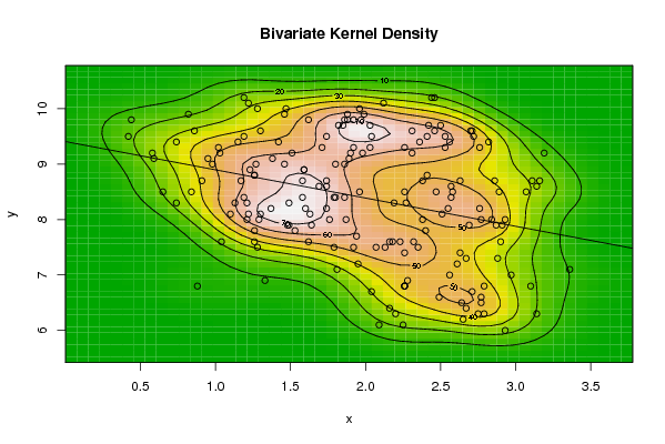
Title produced by software

Bivariate Kernel Density Estimation

Date of computation

Sun, 08 Nov 2009 04:02:31 -0700

Cite this page as follows

Statistical Computations at FreeStatistics.org, Office for Research Development and Education, URL https://freestatistics.org/blog/index.php?v=date/2009/Nov/08/t1257678190fm381y9rsjjvv13.htm/, Retrieved Mon, 29 Apr 2024 09:53:46 +0000

Statistical Computations at FreeStatistics.org, Office for Research Development and Education, URL https://freestatistics.org/blog/index.php?pk=54509, Retrieved Mon, 29 Apr 2024 09:53:46 +0000

QR Codes:

Paste this QR Code to cite your computation.

Original text written by user:

IsPrivate?

No (this computation is public)

User-defined keywords

Estimated Impact

171

Family? (F = Feedback message, R = changed R code, M = changed R Module, P = changed Parameters, D = changed Data)

-       [Bivariate Kernel Density Estimation] [workshop 6] [2009-11-08 11:02:31] [e81f30a5c3daacfe71a556c99a478849] [Current]
-    D    [Bivariate Kernel Density Estimation] [workshop 6] [2009-11-09 19:29:00] [3d8acb8ffdb376c5fec19e610f8198c2] 
-    D      [Bivariate Kernel Density Estimation] [workshop 6] [2009-11-09 19:42:33] [3d8acb8ffdb376c5fec19e610f8198c2] 

Feedback Forum

Post a new message

Dataseries X:

Download CSV

Histogram

Boxplots

2.28
2.26
2.71
2.77
2.77
2.64
2.56
2.07
2.32
2.16
2.23
2.40
2.84
2.77
2.93
2.91
2.69
2.38
2.58
3.19
2.82
2.72
2.53
2.70
2.42
2.50
2.31
2.41
2.56
2.76
2.71
2.44
2.46
2.12
1.99
1.86
1.88
1.82
1.74
1.71
1.38
1.27
1.19
1.28
1.19
1.22
1.47
1.46
1.96
1.88
2.03
2.04
1.90
1.80
1.92
1.92
1.97
2.46
2.36
2.53
2.31
1.98
1.46
1.26
1.58
1.74
1.89
1.85
1.62
1.30
1.42
1.15
0.42
0.74
1.02
1.51
1.86
1.59
1.03
0.44
0.82
0.86
0.58
0.59
0.95
0.98
1.23
1.17
0.84
0.74
0.65
0.91
1.19
1.30
1.53
1.94
1.79
1.95
2.26
2.04
2.16
2.75
2.79
2.88
3.36
2.97
3.10
2.49
2.20
2.25
2.09
2.79
3.14
2.93
2.65
2.67
2.26
2.35
2.13
2.18
2.90
2.63
2.67
1.81
1.33
0.88
1.28
1.26
1.26
1.29
1.10
1.37
1.21
1.74
1.76
1.48
1.04
1.62
1.49
1.79
1.80
1.58
1.86
1.74
1.59
1.26
1.13
1.92
2.61
2.26
2.41
2.26
2.03
2.86
2.55
2.27
2.26
2.57
3.07
2.76
2.51
2.87
3.14
3.11
3.16
2.47
2.57
2.89
2.63
2.38
1.69
1.96
2.19
1.87
1.6
1.63
1.22
1.21
1.49
1.64

Dataseries Y:

Download CSV

Histogram

6.9
6.8
6.7
6.6
6.5
6.5
7.0
7.5
7.6
7.6
7.6
7.8
8.0
8.0
8.0
7.9
7.9
8.0
8.5
9.2
9.4
9.5
9.5
9.6
9.7
9.7
9.6
9.5
9.4
9.3
9.6
10.2
10.2
10.1
9.9
9.8
9.8
9.7
9.5
9.3
9.1
9.0
9.5
10.0
10.2
10.1
10.0
9.9
10.0
9.9
9.7
9.5
9.2
9.0
9.3
9.8
9.8
9.6
9.4
9.3
9.2
9.2
9.0
8.8
8.7
8.7
9.1
9.7
9.8
9.6
9.4
9.4
9.5
9.4
9.3
9.2
9.0
8.9
9.2
9.8
9.9
9.6
9.2
9.1
9.1
9.0
8.9
8.7
8.5
8.3
8.5
8.7
8.4
8.1
7.8
7.7
7.5
7.2
6.8
6.7
6.4
6.3
6.8
7.3
7.1
7.0
6.8
6.6
6.3
6.1
6.1
6.3
6.3
6.0
6.2
6.4
6.8
7.5
7.5
7.6
7.6
7.4
7.3
7.1
6.9
6.8
7.5
7.6
7.8
8.0
8.1
8.2
8.3
8.2
8.0
7.9
7.6
7.6
8.3
8.4
8.4
8.4
8.4
8.6
8.9
8.8
8.3
7.5
7.2
7.4
8.8
9.3
9.3
8.7
8.2
8.3
8.5
8.6
8.5
8.2
8.1
7.9
8.6
8.7
8.7
8.5
8.4
8.5
8.7
8.7
8.6
8.5
8.3
8.0
8.2
8.1
8.1
8.0
7.9
7.9

Summary of computational transaction
Raw Input	view raw input (R code)
Raw Output	view raw output of R engine
Computing time	2 seconds
R Server	'Sir Ronald Aylmer Fisher' @ 193.190.124.24

\begin{tabular}{lllllllll}
\hline
Summary of computational transaction \tabularnewline
Raw Input & view raw input (R code)  \tabularnewline
Raw Output & view raw output of R engine  \tabularnewline
Computing time & 2 seconds \tabularnewline
R Server & 'Sir Ronald Aylmer Fisher' @ 193.190.124.24 \tabularnewline
\hline
\end{tabular}
%Source: https://freestatistics.org/blog/index.php?pk=54509&T=0

[TABLE]
[ROW][C]Summary of computational transaction[/C][/ROW]
[ROW][C]Raw Input[/C][C]view raw input (R code) [/C][/ROW]
[ROW][C]Raw Output[/C][C]view raw output of R engine [/C][/ROW]
[ROW][C]Computing time[/C][C]2 seconds[/C][/ROW]
[ROW][C]R Server[/C][C]'Sir Ronald Aylmer Fisher' @ 193.190.124.24[/C][/ROW]
[/TABLE]
Source: https://freestatistics.org/blog/index.php?pk=54509&T=0

Globally Unique Identifier (entire table): ba.freestatistics.org/blog/index.php?pk=54509&T=0

As an alternative you can also use a QR Code:

The GUIDs for individual cells are displayed in the table below:

Summary of computational transaction
Raw Input	view raw input (R code)
Raw Output	view raw output of R engine
Computing time	2 seconds
R Server	'Sir Ronald Aylmer Fisher' @ 193.190.124.24

Bandwidth
x axis	0.253789400155035
y axis	0.349702577059812
Correlation
correlation used in KDE	-0.317658225704477
correlation(x,y)	-0.317658225704477

\begin{tabular}{lllllllll}
\hline
Bandwidth \tabularnewline
x axis & 0.253789400155035 \tabularnewline
y axis & 0.349702577059812 \tabularnewline
Correlation \tabularnewline
correlation used in KDE & -0.317658225704477 \tabularnewline
correlation(x,y) & -0.317658225704477 \tabularnewline
\hline
\end{tabular}
%Source: https://freestatistics.org/blog/index.php?pk=54509&T=1

[TABLE]
[ROW][C]Bandwidth[/C][/ROW]
[ROW][C]x axis[/C][C]0.253789400155035[/C][/ROW]
[ROW][C]y axis[/C][C]0.349702577059812[/C][/ROW]
[ROW][C]Correlation[/C][/ROW]
[ROW][C]correlation used in KDE[/C][C]-0.317658225704477[/C][/ROW]
[ROW][C]correlation(x,y)[/C][C]-0.317658225704477[/C][/ROW]
[/TABLE]
Source: https://freestatistics.org/blog/index.php?pk=54509&T=1

Globally Unique Identifier (entire table): ba.freestatistics.org/blog/index.php?pk=54509&T=1

As an alternative you can also use a QR Code:

The GUIDs for individual cells are displayed in the table below:

Bandwidth
x axis	0.253789400155035
y axis	0.349702577059812
Correlation
correlation used in KDE	-0.317658225704477
correlation(x,y)	-0.317658225704477

Figure 1

PNG link

Postscript link

PDF link

Parameters (Session):

par1 = 50 ; par2 = 50 ; par3 = 0 ; par4 = 0 ; par5 = 0 ; par6 = Y ; par7 = Y ;

Parameters (R input):

par1 = 50 ; par2 = 50 ; par3 = 0 ; par4 = 0 ; par5 = 0 ; par6 = Y ; par7 = Y ;

R code (references can be found in the software module):

par1 <- as(par1,'numeric')
par2 <- as(par2,'numeric')
par3 <- as(par3,'numeric')
par4 <- as(par4,'numeric')
par5 <- as(par5,'numeric')
library('GenKern')
if (par3==0) par3 <- dpik(x)
if (par4==0) par4 <- dpik(y)
if (par5==0) par5 <- cor(x,y)
if (par1 > 500) par1 <- 500
if (par2 > 500) par2 <- 500
bitmap(file='bidensity.png')
op <- KernSur(x,y, xgridsize=par1, ygridsize=par2, correlation=par5, xbandwidth=par3, ybandwidth=par4)
image(op$xords, op$yords, op$zden, col=terrain.colors(100), axes=TRUE,main=main,xlab=xlab,ylab=ylab)
if (par6=='Y') contour(op$xords, op$yords, op$zden, add=TRUE)
if (par7=='Y') points(x,y)
(r<-lm(y ~ x))
abline(r)
box()
dev.off()
load(file='createtable')
a<-table.start()
a<-table.row.start(a)
a<-table.element(a,'Bandwidth',2,TRUE)
a<-table.row.end(a)
a<-table.row.start(a)
a<-table.element(a,'x axis',header=TRUE)
a<-table.element(a,par3)
a<-table.row.end(a)
a<-table.row.start(a)
a<-table.element(a,'y axis',header=TRUE)
a<-table.element(a,par4)
a<-table.row.end(a)
a<-table.row.start(a)
a<-table.element(a,'Correlation',2,TRUE)
a<-table.row.end(a)
a<-table.row.start(a)
a<-table.element(a,'correlation used in KDE',header=TRUE)
a<-table.element(a,par5)
a<-table.row.end(a)
a<-table.row.start(a)
a<-table.element(a,'correlation(x,y)',header=TRUE)
a<-table.element(a,cor(x,y))
a<-table.row.end(a)
a<-table.end(a)
table.save(a,file='mytable.tab')

Free Statistics

Description of Statistical Computation

Tree of Dependent Computations

Dataset

Tables (Output of Computation)

Figures (Output of Computation)

Input Parameters & R Code