Free Statistics
of Irreproducible Research!
Description of Statistical Computation | |||||||||||||||||||||||||||||||||||||||||||||
|---|---|---|---|---|---|---|---|---|---|---|---|---|---|---|---|---|---|---|---|---|---|---|---|---|---|---|---|---|---|---|---|---|---|---|---|---|---|---|---|---|---|---|---|---|---|
| Author's title | |||||||||||||||||||||||||||||||||||||||||||||
| Author | *The author of this computation has been verified* | ||||||||||||||||||||||||||||||||||||||||||||
| R Software Module | rwasp_boxcoxlin.wasp | ||||||||||||||||||||||||||||||||||||||||||||
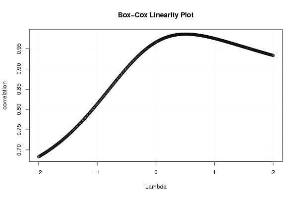
| Title produced by software | Box-Cox Linearity Plot | ||||||||||||||||||||||||||||||||||||||||||||
| Date of computation | Fri, 13 Nov 2009 10:40:29 -0700 | ||||||||||||||||||||||||||||||||||||||||||||
| Cite this page as follows | Statistical Computations at FreeStatistics.org, Office for Research Development and Education, URL https://freestatistics.org/blog/index.php?v=date/2009/Nov/13/t1258134102431hgr1haut69z4.htm/, Retrieved Tue, 28 Jul 2026 14:34:30 +0000 | ||||||||||||||||||||||||||||||||||||||||||||
| Statistical Computations at FreeStatistics.org, Office for Research Development and Education, URL https://freestatistics.org/blog/index.php?pk=56934, Retrieved Tue, 28 Jul 2026 14:34:30 +0000 | |||||||||||||||||||||||||||||||||||||||||||||
| QR Codes: | |||||||||||||||||||||||||||||||||||||||||||||
|
| |||||||||||||||||||||||||||||||||||||||||||||
| Original text written by user: | |||||||||||||||||||||||||||||||||||||||||||||
| IsPrivate? | No (this computation is public) | ||||||||||||||||||||||||||||||||||||||||||||
| User-defined keywords | |||||||||||||||||||||||||||||||||||||||||||||
| Estimated Impact | 510 | ||||||||||||||||||||||||||||||||||||||||||||
Tree of Dependent Computations | |||||||||||||||||||||||||||||||||||||||||||||
| Family? (F = Feedback message, R = changed R code, M = changed R Module, P = changed Parameters, D = changed Data) | |||||||||||||||||||||||||||||||||||||||||||||
| - [Notched Boxplots] [3/11/2009] [2009-11-02 21:10:41] [b98453cac15ba1066b407e146608df68] - PD [Notched Boxplots] [WS 4: Notched Box...] [2009-11-09 12:07:49] [74be16979710d4c4e7c6647856088456] - [Notched Boxplots] [WS 6: Notched Box...] [2009-11-09 12:18:05] [74be16979710d4c4e7c6647856088456] - D [Notched Boxplots] [WS 6 notched boxp...] [2009-11-13 16:51:53] [95cead3ebb75668735f848316249436a] - RMPD [Box-Cox Linearity Plot] [ws6 box-cox] [2009-11-13 17:40:29] [95523ebdb89b97dbf680ec91e0b4bca2] [Current] | |||||||||||||||||||||||||||||||||||||||||||||
| Feedback Forum | |||||||||||||||||||||||||||||||||||||||||||||
Post a new message | |||||||||||||||||||||||||||||||||||||||||||||
Dataset | |||||||||||||||||||||||||||||||||||||||||||||
| Dataseries X: | |||||||||||||||||||||||||||||||||||||||||||||
1.00 1.00 1.00 1.00 1.00 1.00 1.00 1.00 1.00 1.00 1.00 1.00 1.00 1.00 1.00 1.25 1.25 1.25 1.50 1.50 1.50 1.75 1.75 2.00 2.00 2.25 2.25 2.50 2.50 2.50 2.75 2.75 2.75 3.00 3.00 3.00 3.00 3.00 3.00 3.00 3.00 3.00 3.00 3.00 3.00 3.00 3.25 3.25 3.25 3.25 2.75 2.00 1.00 1.00 0.50 0.25 0.25 0.25 0.25 0.25 | |||||||||||||||||||||||||||||||||||||||||||||
| Dataseries Y: | |||||||||||||||||||||||||||||||||||||||||||||
2.05 2.11 2.09 2.05 2.08 2.06 2.06 2.08 2.07 2.06 2.07 2.06 2.09 2.07 2.09 2.28 2.33 2.35 2.52 2.63 2.58 2.70 2.81 2.97 3.04 3.28 3.33 3.50 3.56 3.57 3.69 3.82 3.79 3.96 4.06 4.05 4.03 3.94 4.02 3.88 4.02 4.03 4.09 3.99 4.01 4.01 4.19 4.30 4.27 3.82 3.15 2.49 1.81 1.26 1.06 0.84 0.78 0.70 0.36 0.35 | |||||||||||||||||||||||||||||||||||||||||||||
Tables (Output of Computation) | |||||||||||||||||||||||||||||||||||||||||||||
| |||||||||||||||||||||||||||||||||||||||||||||
Figures (Output of Computation) | |||||||||||||||||||||||||||||||||||||||||||||
Input Parameters & R Code | |||||||||||||||||||||||||||||||||||||||||||||
| Parameters (Session): | |||||||||||||||||||||||||||||||||||||||||||||
| Parameters (R input): | |||||||||||||||||||||||||||||||||||||||||||||
| R code (references can be found in the software module): | |||||||||||||||||||||||||||||||||||||||||||||
n <- length(x) | |||||||||||||||||||||||||||||||||||||||||||||