Repository of Reproducible Computations

Free Statistics

of Irreproducible Research!

Author's title

Author

*The author of this computation has been verified*

R Software Module

rwasp_notchedbox1.wasp

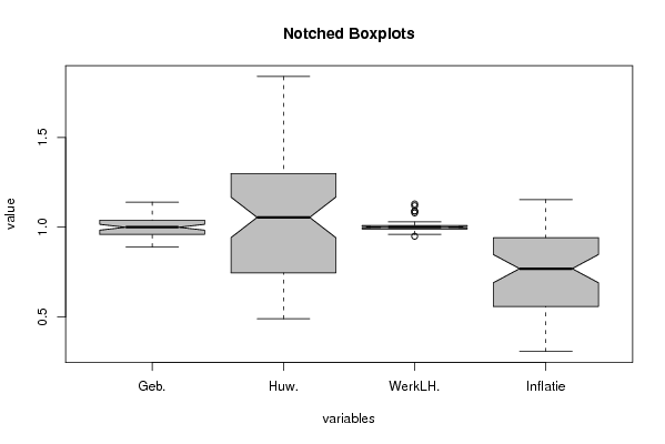
Title produced by software

Notched Boxplots

Date of computation

Fri, 20 Nov 2009 07:01:16 -0700

Cite this page as follows

Statistical Computations at FreeStatistics.org, Office for Research Development and Education, URL https://freestatistics.org/blog/index.php?v=date/2009/Nov/20/t1258725847phv8ewhvhdyyz5v.htm/, Retrieved Tue, 30 Apr 2024 14:34:39 +0000

Statistical Computations at FreeStatistics.org, Office for Research Development and Education, URL https://freestatistics.org/blog/index.php?pk=58173, Retrieved Tue, 30 Apr 2024 14:34:39 +0000

QR Codes:

Paste this QR Code to cite your computation.

Original text written by user:

IsPrivate?

No (this computation is public)

User-defined keywords

Estimated Impact

145

Family? (F = Feedback message, R = changed R code, M = changed R Module, P = changed Parameters, D = changed Data)

-     [Notched Boxplots] [WS6 Boxplot alle ...] [2009-11-09 20:21:51] [1b4c3bbe3f2ba180dd536c5a6a81a8e6]
-    D    [Notched Boxplots] [] [2009-11-20 14:01:16] [51118f1042b56b16d340924f16263174] [Current]
-    D      [Notched Boxplots] [] [2009-11-20 14:21:07] [830e13ac5e5ac1e5b21c6af0c149b21d] 

Feedback Forum

Post a new message

Dataseries X:

Download CSV

Histogram

Boxplots

1	1	1	1
0,92	1,84	1	0,961538462
1,11	1,04	0,99	0,961538462
1	1,19	0,98	0,615384615
1,04	1,62	0,99	0,538461538
0,95	1,23	1	0,307692308
1	0,83	1,13	0,423076923
0,97	1,43	1,02	0,5
0,97	0,72	1	0,461538462
1,03	0,66	0,99	0,5
0,9	0,62	0,98	0,423076923
1,07	1,1	1,01	0,5
1,04	0,65	1,01	0,461538462
0,89	1,64	1	0,615384615
1,07	1,11	0,99	0,653846154
1,03	1,23	1	0,576923077
0,96	1,58	0,98	0,346153846
1,02	1,04	1,01	0,576923077
1,1	0,93	1,12	0,538461538
0,93	1,36	1,02	0,615384615
1,02	0,77	1	0,653846154
0,98	0,66	0,98	0,538461538
0,93	0,61	0,97	0,692307692
1,09	1,17	1,01	0,653846154
1,01	0,72	1,01	0,538461538
0,93	1,55	1	0,461538462
1,07	0,9	0,99	0,384615385
0,95	1,62	0,98	0,653846154
0,99	1,3	0,99	0,923076923
1,08	1,06	1,01	0,769230769
1,05	1,16	1,09	0,807692308
0,98	0,95	1,03	0,769230769
0,98	0,91	1	0,692307692
0,98	0,65	1	1,038461538
0,96	0,62	0,97	0,884615385
1,07	1,15	1	0,730769231
0,98	0,69	0,99	0,769230769
0,93	1,34	1	0,884615385
1,13	1,04	0,99	1,076923077
0,95	1,64	0,98	0,923076923
1,01	1,3	0,99	0,884615385
1,01	1,05	1	1,038461538
1,01	1,19	1,09	1,038461538
1,04	0,96	1,01	1,115384615
0,97	0,95	1	1,153846154
1	0,58	0,97	0,846153846
0,92	0,65	0,97	0,884615385
1,06	1,15	1	1,076923077
1,03	0,65	0,99	1,076923077
0,9	1,32	0,99	1,076923077
1,14	1,25	0,98	0,846153846
0,93	1,4	0,99	1
1,08	1,33	1	1,076923077
0,98	1,2	1	0,961538462
1,02	1	1,08	0,923076923
1,02	1,03	1,01	0,884615385
1	1,07	0,99	0,730769231
1,01	0,49	0,95	0,653846154
0,91	0,64	0,96	0,769230769
0,98	1,32	0,99	0,807692308

Summary of computational transaction
Raw Input	view raw input (R code)
Raw Output	view raw output of R engine
Computing time	1 seconds
R Server	'Gwilym Jenkins' @ 72.249.127.135

\begin{tabular}{lllllllll}
\hline
Summary of computational transaction \tabularnewline
Raw Input & view raw input (R code)  \tabularnewline
Raw Output & view raw output of R engine  \tabularnewline
Computing time & 1 seconds \tabularnewline
R Server & 'Gwilym Jenkins' @ 72.249.127.135 \tabularnewline
\hline
\end{tabular}
%Source: https://freestatistics.org/blog/index.php?pk=58173&T=0

[TABLE]
[ROW][C]Summary of computational transaction[/C][/ROW]
[ROW][C]Raw Input[/C][C]view raw input (R code) [/C][/ROW]
[ROW][C]Raw Output[/C][C]view raw output of R engine [/C][/ROW]
[ROW][C]Computing time[/C][C]1 seconds[/C][/ROW]
[ROW][C]R Server[/C][C]'Gwilym Jenkins' @ 72.249.127.135[/C][/ROW]
[/TABLE]
Source: https://freestatistics.org/blog/index.php?pk=58173&T=0

Globally Unique Identifier (entire table): ba.freestatistics.org/blog/index.php?pk=58173&T=0

As an alternative you can also use a QR Code:

The GUIDs for individual cells are displayed in the table below:

Summary of computational transaction
Raw Input	view raw input (R code)
Raw Output	view raw output of R engine
Computing time	1 seconds
R Server	'Gwilym Jenkins' @ 72.249.127.135

Boxplot statistics
Variable	lower whisker	lower hinge	median	upper hinge	upper whisker
Geb.	0.89	0.96	1	1.04	1.14
Huw.	0.49	0.745	1.055	1.3	1.84
WerkLH.	0.96	0.99	1	1.01	1.03
Inflatie	0.307692308	0.5576923075	0.769230769	0.9423076925	1.153846154

\begin{tabular}{lllllllll}
\hline
Boxplot statistics \tabularnewline
Variable & lower whisker & lower hinge & median & upper hinge & upper whisker \tabularnewline
Geb. & 0.89 & 0.96 & 1 & 1.04 & 1.14 \tabularnewline
Huw. & 0.49 & 0.745 & 1.055 & 1.3 & 1.84 \tabularnewline
WerkLH. & 0.96 & 0.99 & 1 & 1.01 & 1.03 \tabularnewline
Inflatie & 0.307692308 & 0.5576923075 & 0.769230769 & 0.9423076925 & 1.153846154 \tabularnewline
\hline
\end{tabular}
%Source: https://freestatistics.org/blog/index.php?pk=58173&T=1

[TABLE]
[ROW][C]Boxplot statistics[/C][/ROW]
[ROW][C]Variable[/C][C]lower whisker[/C][C]lower hinge[/C][C]median[/C][C]upper hinge[/C][C]upper whisker[/C][/ROW]
[ROW][C]Geb.[/C][C]0.89[/C][C]0.96[/C][C]1[/C][C]1.04[/C][C]1.14[/C][/ROW]
[ROW][C]Huw.[/C][C]0.49[/C][C]0.745[/C][C]1.055[/C][C]1.3[/C][C]1.84[/C][/ROW]
[ROW][C]WerkLH.[/C][C]0.96[/C][C]0.99[/C][C]1[/C][C]1.01[/C][C]1.03[/C][/ROW]
[ROW][C]Inflatie[/C][C]0.307692308[/C][C]0.5576923075[/C][C]0.769230769[/C][C]0.9423076925[/C][C]1.153846154[/C][/ROW]
[/TABLE]
Source: https://freestatistics.org/blog/index.php?pk=58173&T=1

Globally Unique Identifier (entire table): ba.freestatistics.org/blog/index.php?pk=58173&T=1

As an alternative you can also use a QR Code:

The GUIDs for individual cells are displayed in the table below:

Boxplot statistics
Variable	lower whisker	lower hinge	median	upper hinge	upper whisker
Geb.	0.89	0.96	1	1.04	1.14
Huw.	0.49	0.745	1.055	1.3	1.84
WerkLH.	0.96	0.99	1	1.01	1.03
Inflatie	0.307692308	0.5576923075	0.769230769	0.9423076925	1.153846154

Boxplot Notches
Variable	lower bound	median	upper bound
Geb.	0.98368183016798	1	1.01631816983202
Huw.	0.941792696790357	1.055	1.16820730320964
WerkLH.	0.995920457541995	1	1.00407954245801
Inflatie	0.690778029344525	0.769230769	0.847683508655475

\begin{tabular}{lllllllll}
\hline
Boxplot Notches \tabularnewline
Variable & lower bound & median & upper bound \tabularnewline
Geb. & 0.98368183016798 & 1 & 1.01631816983202 \tabularnewline
Huw. & 0.941792696790357 & 1.055 & 1.16820730320964 \tabularnewline
WerkLH. & 0.995920457541995 & 1 & 1.00407954245801 \tabularnewline
Inflatie & 0.690778029344525 & 0.769230769 & 0.847683508655475 \tabularnewline
\hline
\end{tabular}
%Source: https://freestatistics.org/blog/index.php?pk=58173&T=2

[TABLE]
[ROW][C]Boxplot Notches[/C][/ROW]
[ROW][C]Variable[/C][C]lower bound[/C][C]median[/C][C]upper bound[/C][/ROW]
[ROW][C]Geb.[/C][C]0.98368183016798[/C][C]1[/C][C]1.01631816983202[/C][/ROW]
[ROW][C]Huw.[/C][C]0.941792696790357[/C][C]1.055[/C][C]1.16820730320964[/C][/ROW]
[ROW][C]WerkLH.[/C][C]0.995920457541995[/C][C]1[/C][C]1.00407954245801[/C][/ROW]
[ROW][C]Inflatie[/C][C]0.690778029344525[/C][C]0.769230769[/C][C]0.847683508655475[/C][/ROW]
[/TABLE]
Source: https://freestatistics.org/blog/index.php?pk=58173&T=2

Globally Unique Identifier (entire table): ba.freestatistics.org/blog/index.php?pk=58173&T=2

As an alternative you can also use a QR Code:

The GUIDs for individual cells are displayed in the table below:

Boxplot Notches
Variable	lower bound	median	upper bound
Geb.	0.98368183016798	1	1.01631816983202
Huw.	0.941792696790357	1.055	1.16820730320964
WerkLH.	0.995920457541995	1	1.00407954245801
Inflatie	0.690778029344525	0.769230769	0.847683508655475

Figure 1

PNG link

Postscript link

PDF link

Parameters (Session):

par1 = grey ;

Parameters (R input):

par1 = grey ;

R code (references can be found in the software module):

z <- as.data.frame(t(y))
bitmap(file='test1.png')
(r<-boxplot(z ,xlab=xlab,ylab=ylab,main=main,notch=TRUE,col=par1))
dev.off()
load(file='createtable')
a<-table.start()
a<-table.row.start(a)
a<-table.element(a,hyperlink('overview.htm','Boxplot statistics','Boxplot overview'),6,TRUE)
a<-table.row.end(a)
a<-table.row.start(a)
a<-table.element(a,'Variable',1,TRUE)
a<-table.element(a,hyperlink('lower_whisker.htm','lower whisker','definition of lower whisker'),1,TRUE)
a<-table.element(a,hyperlink('lower_hinge.htm','lower hinge','definition of lower hinge'),1,TRUE)
a<-table.element(a,hyperlink('central_tendency.htm','median','definitions about measures of central tendency'),1,TRUE)
a<-table.element(a,hyperlink('upper_hinge.htm','upper hinge','definition of upper hinge'),1,TRUE)
a<-table.element(a,hyperlink('upper_whisker.htm','upper whisker','definition of upper whisker'),1,TRUE)
a<-table.row.end(a)
for (i in 1:length(y[,1]))
{
a<-table.row.start(a)
a<-table.element(a,dimnames(t(x))[[2]][i],1,TRUE)
for (j in 1:5)
{
a<-table.element(a,r$stats[j,i])
}
a<-table.row.end(a)
}
a<-table.end(a)
table.save(a,file='mytable.tab')
a<-table.start()
a<-table.row.start(a)
a<-table.element(a,'Boxplot Notches',4,TRUE)
a<-table.row.end(a)
a<-table.row.start(a)
a<-table.element(a,'Variable',1,TRUE)
a<-table.element(a,'lower bound',1,TRUE)
a<-table.element(a,'median',1,TRUE)
a<-table.element(a,'upper bound',1,TRUE)
a<-table.row.end(a)
for (i in 1:length(y[,1]))
{
a<-table.row.start(a)
a<-table.element(a,dimnames(t(x))[[2]][i],1,TRUE)
a<-table.element(a,r$conf[1,i])
a<-table.element(a,r$stats[3,i])
a<-table.element(a,r$conf[2,i])
a<-table.row.end(a)
}
a<-table.end(a)
table.save(a,file='mytable1.tab')

Free Statistics

Description of Statistical Computation

Tree of Dependent Computations

Dataset

Tables (Output of Computation)

Figures (Output of Computation)

Input Parameters & R Code