Repository of Reproducible Computations

Free Statistics

of Irreproducible Research!

Author's title

Author

*The author of this computation has been verified*

R Software Module

rwasp_autocorrelation.wasp

Title produced by software

(Partial) Autocorrelation Function

Date of computation

Sat, 28 Nov 2009 11:28:34 -0700

Cite this page as follows

Statistical Computations at FreeStatistics.org, Office for Research Development and Education, URL https://freestatistics.org/blog/index.php?v=date/2009/Nov/28/t1259433024fooln9fzi0fndlt.htm/, Retrieved Sat, 26 Sep 2026 09:44:16 +0000

Statistical Computations at FreeStatistics.org, Office for Research Development and Education, URL https://freestatistics.org/blog/index.php?pk=61519, Retrieved Sat, 26 Sep 2026 09:44:16 +0000

QR Codes:

Paste this QR Code to cite your computation.

Original text written by user:

IsPrivate?

No (this computation is public)

User-defined keywords

Estimated Impact

499

Family? (F = Feedback message, R = changed R code, M = changed R Module, P = changed Parameters, D = changed Data)

F       [(Partial) Autocorrelation Function] [] [2009-11-28 18:28:34] [aef022288383377281176d9807aba5bf] [Current]
- R P     [(Partial) Autocorrelation Function] [Review WS 8] [2009-12-01 20:55:58] [1f74ef2f756548f1f3a7b6136ea56d7f] 

Feedback Forum

2009-12-04 13:07:29 [Angelo Stuer] [reply] 
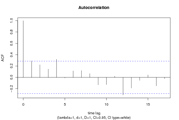
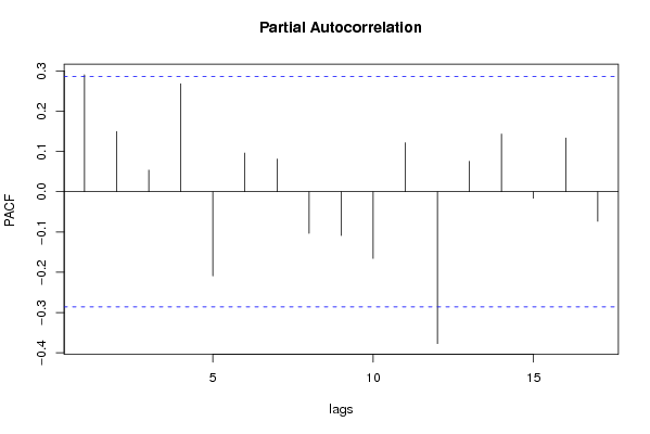
Let op dat je niet te veel differentieert. Je ziet duidelijk dat het seizoenaal differentiëren niks verandert aan de tijdreeks dus is het ook niet nodig dit te doen.

Post a new message

Dataseries X:

Download CSV

Histogram

Boxplots

Summary of computational transaction
Raw Input	view raw input (R code)
Raw Output	view raw output of R engine
Computing time	1 seconds
R Server	'Gwilym Jenkins' @ 72.249.127.135

\begin{tabular}{lllllllll}
\hline
Summary of computational transaction \tabularnewline
Raw Input & view raw input (R code)  \tabularnewline
Raw Output & view raw output of R engine  \tabularnewline
Computing time & 1 seconds \tabularnewline
R Server & 'Gwilym Jenkins' @ 72.249.127.135 \tabularnewline
\hline
\end{tabular}
%Source: https://freestatistics.org/blog/index.php?pk=61519&T=0

[TABLE]
[ROW][C]Summary of computational transaction[/C][/ROW]
[ROW][C]Raw Input[/C][C]view raw input (R code) [/C][/ROW]
[ROW][C]Raw Output[/C][C]view raw output of R engine [/C][/ROW]
[ROW][C]Computing time[/C][C]1 seconds[/C][/ROW]
[ROW][C]R Server[/C][C]'Gwilym Jenkins' @ 72.249.127.135[/C][/ROW]
[/TABLE]
Source: https://freestatistics.org/blog/index.php?pk=61519&T=0

Globally Unique Identifier (entire table): ba.freestatistics.org/blog/index.php?pk=61519&T=0

As an alternative you can also use a QR Code:

The GUIDs for individual cells are displayed in the table below:

Summary of computational transaction
Raw Input	view raw input (R code)
Raw Output	view raw output of R engine
Computing time	1 seconds
R Server	'Gwilym Jenkins' @ 72.249.127.135

Autocorrelation Function
Time lag k	ACF(k)	T-STAT	P-value
1	0.290187	1.9894	0.026246
2	0.221189	1.5164	0.068059
3	0.145977	1.0008	0.161032
4	0.319801	2.1924	0.016667
5	-0.011316	-0.0776	0.469247
6	0.114614	0.7858	0.217977
7	0.120652	0.8271	0.206167
8	0.06642	0.4554	0.325477
9	-0.13234	-0.9073	0.184445
10	-0.12855	-0.8813	0.191322
11	0.019875	0.1363	0.4461
12	-0.311101	-2.1328	0.019097
13	-0.188652	-1.2933	0.101108
14	-0.053904	-0.3696	0.356689
15	0.043144	0.2958	0.384351
16	-0.149696	-1.0263	0.155011
17	-0.023376	-0.1603	0.436682

\begin{tabular}{lllllllll}
\hline
Autocorrelation Function \tabularnewline
Time lag k & ACF(k) & T-STAT & P-value \tabularnewline
1 & 0.290187 & 1.9894 & 0.026246 \tabularnewline
2 & 0.221189 & 1.5164 & 0.068059 \tabularnewline
3 & 0.145977 & 1.0008 & 0.161032 \tabularnewline
4 & 0.319801 & 2.1924 & 0.016667 \tabularnewline
5 & -0.011316 & -0.0776 & 0.469247 \tabularnewline
6 & 0.114614 & 0.7858 & 0.217977 \tabularnewline
7 & 0.120652 & 0.8271 & 0.206167 \tabularnewline
8 & 0.06642 & 0.4554 & 0.325477 \tabularnewline
9 & -0.13234 & -0.9073 & 0.184445 \tabularnewline
10 & -0.12855 & -0.8813 & 0.191322 \tabularnewline
11 & 0.019875 & 0.1363 & 0.4461 \tabularnewline
12 & -0.311101 & -2.1328 & 0.019097 \tabularnewline
13 & -0.188652 & -1.2933 & 0.101108 \tabularnewline
14 & -0.053904 & -0.3696 & 0.356689 \tabularnewline
15 & 0.043144 & 0.2958 & 0.384351 \tabularnewline
16 & -0.149696 & -1.0263 & 0.155011 \tabularnewline
17 & -0.023376 & -0.1603 & 0.436682 \tabularnewline
\hline
\end{tabular}
%Source: https://freestatistics.org/blog/index.php?pk=61519&T=1

[TABLE]
[ROW][C]Autocorrelation Function[/C][/ROW]
[ROW][C]Time lag k[/C][C]ACF(k)[/C][C]T-STAT[/C][C]P-value[/C][/ROW]
[ROW][C]1[/C][C]0.290187[/C][C]1.9894[/C][C]0.026246[/C][/ROW]
[ROW][C]2[/C][C]0.221189[/C][C]1.5164[/C][C]0.068059[/C][/ROW]
[ROW][C]3[/C][C]0.145977[/C][C]1.0008[/C][C]0.161032[/C][/ROW]
[ROW][C]4[/C][C]0.319801[/C][C]2.1924[/C][C]0.016667[/C][/ROW]
[ROW][C]5[/C][C]-0.011316[/C][C]-0.0776[/C][C]0.469247[/C][/ROW]
[ROW][C]6[/C][C]0.114614[/C][C]0.7858[/C][C]0.217977[/C][/ROW]
[ROW][C]7[/C][C]0.120652[/C][C]0.8271[/C][C]0.206167[/C][/ROW]
[ROW][C]8[/C][C]0.06642[/C][C]0.4554[/C][C]0.325477[/C][/ROW]
[ROW][C]9[/C][C]-0.13234[/C][C]-0.9073[/C][C]0.184445[/C][/ROW]
[ROW][C]10[/C][C]-0.12855[/C][C]-0.8813[/C][C]0.191322[/C][/ROW]
[ROW][C]11[/C][C]0.019875[/C][C]0.1363[/C][C]0.4461[/C][/ROW]
[ROW][C]12[/C][C]-0.311101[/C][C]-2.1328[/C][C]0.019097[/C][/ROW]
[ROW][C]13[/C][C]-0.188652[/C][C]-1.2933[/C][C]0.101108[/C][/ROW]
[ROW][C]14[/C][C]-0.053904[/C][C]-0.3696[/C][C]0.356689[/C][/ROW]
[ROW][C]15[/C][C]0.043144[/C][C]0.2958[/C][C]0.384351[/C][/ROW]
[ROW][C]16[/C][C]-0.149696[/C][C]-1.0263[/C][C]0.155011[/C][/ROW]
[ROW][C]17[/C][C]-0.023376[/C][C]-0.1603[/C][C]0.436682[/C][/ROW]
[/TABLE]
Source: https://freestatistics.org/blog/index.php?pk=61519&T=1

Globally Unique Identifier (entire table): ba.freestatistics.org/blog/index.php?pk=61519&T=1

As an alternative you can also use a QR Code:

The GUIDs for individual cells are displayed in the table below:

Autocorrelation Function
Time lag k	ACF(k)	T-STAT	P-value
1	0.290187	1.9894	0.026246
2	0.221189	1.5164	0.068059
3	0.145977	1.0008	0.161032
4	0.319801	2.1924	0.016667
5	-0.011316	-0.0776	0.469247
6	0.114614	0.7858	0.217977
7	0.120652	0.8271	0.206167
8	0.06642	0.4554	0.325477
9	-0.13234	-0.9073	0.184445
10	-0.12855	-0.8813	0.191322
11	0.019875	0.1363	0.4461
12	-0.311101	-2.1328	0.019097
13	-0.188652	-1.2933	0.101108
14	-0.053904	-0.3696	0.356689
15	0.043144	0.2958	0.384351
16	-0.149696	-1.0263	0.155011
17	-0.023376	-0.1603	0.436682

Partial Autocorrelation Function
Time lag k	PACF(k)	T-STAT	P-value
1	0.290187	1.9894	0.026246
2	0.149576	1.0254	0.155202
3	0.053598	0.3674	0.357466
4	0.26798	1.8372	0.036255
5	-0.208922	-1.4323	0.079339
6	0.095925	0.6576	0.256993
7	0.08111	0.5561	0.290404
8	-0.103306	-0.7082	0.241149
9	-0.108833	-0.7461	0.229654
10	-0.165488	-1.1345	0.131164
11	0.121584	0.8335	0.204379
12	-0.376967	-2.5844	0.006461
13	0.075324	0.5164	0.304
14	0.143119	0.9812	0.165765
15	-0.016065	-0.1101	0.456386
16	0.133173	0.913	0.182955
17	-0.073251	-0.5022	0.308941

\begin{tabular}{lllllllll}
\hline
Partial Autocorrelation Function \tabularnewline
Time lag k & PACF(k) & T-STAT & P-value \tabularnewline
1 & 0.290187 & 1.9894 & 0.026246 \tabularnewline
2 & 0.149576 & 1.0254 & 0.155202 \tabularnewline
3 & 0.053598 & 0.3674 & 0.357466 \tabularnewline
4 & 0.26798 & 1.8372 & 0.036255 \tabularnewline
5 & -0.208922 & -1.4323 & 0.079339 \tabularnewline
6 & 0.095925 & 0.6576 & 0.256993 \tabularnewline
7 & 0.08111 & 0.5561 & 0.290404 \tabularnewline
8 & -0.103306 & -0.7082 & 0.241149 \tabularnewline
9 & -0.108833 & -0.7461 & 0.229654 \tabularnewline
10 & -0.165488 & -1.1345 & 0.131164 \tabularnewline
11 & 0.121584 & 0.8335 & 0.204379 \tabularnewline
12 & -0.376967 & -2.5844 & 0.006461 \tabularnewline
13 & 0.075324 & 0.5164 & 0.304 \tabularnewline
14 & 0.143119 & 0.9812 & 0.165765 \tabularnewline
15 & -0.016065 & -0.1101 & 0.456386 \tabularnewline
16 & 0.133173 & 0.913 & 0.182955 \tabularnewline
17 & -0.073251 & -0.5022 & 0.308941 \tabularnewline
\hline
\end{tabular}
%Source: https://freestatistics.org/blog/index.php?pk=61519&T=2

[TABLE]
[ROW][C]Partial Autocorrelation Function[/C][/ROW]
[ROW][C]Time lag k[/C][C]PACF(k)[/C][C]T-STAT[/C][C]P-value[/C][/ROW]
[ROW][C]1[/C][C]0.290187[/C][C]1.9894[/C][C]0.026246[/C][/ROW]
[ROW][C]2[/C][C]0.149576[/C][C]1.0254[/C][C]0.155202[/C][/ROW]
[ROW][C]3[/C][C]0.053598[/C][C]0.3674[/C][C]0.357466[/C][/ROW]
[ROW][C]4[/C][C]0.26798[/C][C]1.8372[/C][C]0.036255[/C][/ROW]
[ROW][C]5[/C][C]-0.208922[/C][C]-1.4323[/C][C]0.079339[/C][/ROW]
[ROW][C]6[/C][C]0.095925[/C][C]0.6576[/C][C]0.256993[/C][/ROW]
[ROW][C]7[/C][C]0.08111[/C][C]0.5561[/C][C]0.290404[/C][/ROW]
[ROW][C]8[/C][C]-0.103306[/C][C]-0.7082[/C][C]0.241149[/C][/ROW]
[ROW][C]9[/C][C]-0.108833[/C][C]-0.7461[/C][C]0.229654[/C][/ROW]
[ROW][C]10[/C][C]-0.165488[/C][C]-1.1345[/C][C]0.131164[/C][/ROW]
[ROW][C]11[/C][C]0.121584[/C][C]0.8335[/C][C]0.204379[/C][/ROW]
[ROW][C]12[/C][C]-0.376967[/C][C]-2.5844[/C][C]0.006461[/C][/ROW]
[ROW][C]13[/C][C]0.075324[/C][C]0.5164[/C][C]0.304[/C][/ROW]
[ROW][C]14[/C][C]0.143119[/C][C]0.9812[/C][C]0.165765[/C][/ROW]
[ROW][C]15[/C][C]-0.016065[/C][C]-0.1101[/C][C]0.456386[/C][/ROW]
[ROW][C]16[/C][C]0.133173[/C][C]0.913[/C][C]0.182955[/C][/ROW]
[ROW][C]17[/C][C]-0.073251[/C][C]-0.5022[/C][C]0.308941[/C][/ROW]
[/TABLE]
Source: https://freestatistics.org/blog/index.php?pk=61519&T=2

Globally Unique Identifier (entire table): ba.freestatistics.org/blog/index.php?pk=61519&T=2

As an alternative you can also use a QR Code:

The GUIDs for individual cells are displayed in the table below:

Partial Autocorrelation Function
Time lag k	PACF(k)	T-STAT	P-value
1	0.290187	1.9894	0.026246
2	0.149576	1.0254	0.155202
3	0.053598	0.3674	0.357466
4	0.26798	1.8372	0.036255
5	-0.208922	-1.4323	0.079339
6	0.095925	0.6576	0.256993
7	0.08111	0.5561	0.290404
8	-0.103306	-0.7082	0.241149
9	-0.108833	-0.7461	0.229654
10	-0.165488	-1.1345	0.131164
11	0.121584	0.8335	0.204379
12	-0.376967	-2.5844	0.006461
13	0.075324	0.5164	0.304
14	0.143119	0.9812	0.165765
15	-0.016065	-0.1101	0.456386
16	0.133173	0.913	0.182955
17	-0.073251	-0.5022	0.308941

Figure 1

PNG link

Postscript link

PDF link

Figure 2

PNG link

Postscript link

PDF link

Parameters (Session):

par1 = Default ; par2 = 1 ; par3 = 1 ; par4 = 1 ; par5 = 12 ; par6 = White Noise ; par7 = 0.95 ;

Parameters (R input):

par1 = Default ; par2 = 1 ; par3 = 1 ; par4 = 1 ; par5 = 12 ; par6 = White Noise ; par7 = 0.95 ;

R code (references can be found in the software module):

if (par1 == 'Default') {
par1 = 10*log10(length(x))
} else {
par1 <- as.numeric(par1)
}
par2 <- as.numeric(par2)
par3 <- as.numeric(par3)
par4 <- as.numeric(par4)
par5 <- as.numeric(par5)
if (par6 == 'White Noise') par6 <- 'white' else par6 <- 'ma'
par7 <- as.numeric(par7)
if (par2 == 0) {
x <- log(x)
} else {
x <- (x ^ par2 - 1) / par2
}
if (par3 > 0) x <- diff(x,lag=1,difference=par3)
if (par4 > 0) x <- diff(x,lag=par5,difference=par4)
bitmap(file='pic1.png')
racf <- acf(x, par1, main='Autocorrelation', xlab='time lag', ylab='ACF', ci.type=par6, ci=par7, sub=paste('(lambda=',par2,', d=',par3,', D=',par4,', CI=', par7, ', CI type=',par6,')',sep=''))
dev.off()
bitmap(file='pic2.png')
rpacf <- pacf(x,par1,main='Partial Autocorrelation',xlab='lags',ylab='PACF')
dev.off()
(myacf <- c(racf$acf))
(mypacf <- c(rpacf$acf))
lengthx <- length(x)
sqrtn <- sqrt(lengthx)
load(file='createtable')
a<-table.start()
a<-table.row.start(a)
a<-table.element(a,'Autocorrelation Function',4,TRUE)
a<-table.row.end(a)
a<-table.row.start(a)
a<-table.element(a,'Time lag k',header=TRUE)
a<-table.element(a,hyperlink('basics.htm','ACF(k)','click here for more information about the Autocorrelation Function'),header=TRUE)
a<-table.element(a,'T-STAT',header=TRUE)
a<-table.element(a,'P-value',header=TRUE)
a<-table.row.end(a)
for (i in 2:(par1+1)) {
a<-table.row.start(a)
a<-table.element(a,i-1,header=TRUE)
a<-table.element(a,round(myacf[i],6))
mytstat <- myacf[i]*sqrtn
a<-table.element(a,round(mytstat,4))
a<-table.element(a,round(1-pt(abs(mytstat),lengthx),6))
a<-table.row.end(a)
}
a<-table.end(a)
table.save(a,file='mytable.tab')
a<-table.start()
a<-table.row.start(a)
a<-table.element(a,'Partial Autocorrelation Function',4,TRUE)
a<-table.row.end(a)
a<-table.row.start(a)
a<-table.element(a,'Time lag k',header=TRUE)
a<-table.element(a,hyperlink('basics.htm','PACF(k)','click here for more information about the Partial Autocorrelation Function'),header=TRUE)
a<-table.element(a,'T-STAT',header=TRUE)
a<-table.element(a,'P-value',header=TRUE)
a<-table.row.end(a)
for (i in 1:par1) {
a<-table.row.start(a)
a<-table.element(a,i,header=TRUE)
a<-table.element(a,round(mypacf[i],6))
mytstat <- mypacf[i]*sqrtn
a<-table.element(a,round(mytstat,4))
a<-table.element(a,round(1-pt(abs(mytstat),lengthx),6))
a<-table.row.end(a)
}
a<-table.end(a)
table.save(a,file='mytable1.tab')

Free Statistics

Description of Statistical Computation

Tree of Dependent Computations

Dataset

Tables (Output of Computation)

Figures (Output of Computation)

Input Parameters & R Code