Repository of Reproducible Computations

Free Statistics

of Irreproducible Research!

Author's title

Author

*The author of this computation has been verified*

R Software Module

rwasp_autocorrelation.wasp

Title produced by software

(Partial) Autocorrelation Function

Date of computation

Thu, 16 Dec 2010 18:44:05 +0000

Cite this page as follows

Statistical Computations at FreeStatistics.org, Office for Research Development and Education, URL https://freestatistics.org/blog/index.php?v=date/2010/Dec/16/t1292524913cwpokqxzc25mio8.htm/, Retrieved Tue, 30 Apr 2024 03:03:40 +0000

Statistical Computations at FreeStatistics.org, Office for Research Development and Education, URL https://freestatistics.org/blog/index.php?pk=111170, Retrieved Tue, 30 Apr 2024 03:03:40 +0000

QR Codes:

Paste this QR Code to cite your computation.

Original text written by user:

IsPrivate?

No (this computation is public)

User-defined keywords

Estimated Impact

167

Family? (F = Feedback message, R = changed R code, M = changed R Module, P = changed Parameters, D = changed Data)

-     [Multiple Regression] [Q1 The Seatbeltlaw] [2007-11-14 19:27:43] [8cd6641b921d30ebe00b648d1481bba0]
- RMPD  [Multiple Regression] [Seatbelt] [2009-11-12 13:54:52] [b98453cac15ba1066b407e146608df68]
-    D    [Multiple Regression] [WS7] [2009-11-18 17:01:04] [8b1aef4e7013bd33fbc2a5833375c5f5]
-   PD      [Multiple Regression] [WS7(2)] [2009-11-20 19:01:46] [7d268329e554b8694908ba13e6e6f258]
-   P         [Multiple Regression] [WS7(3)] [2009-11-21 10:22:47] [7d268329e554b8694908ba13e6e6f258]
-   PD          [Multiple Regression] [WS7(4)] [2009-11-21 10:55:20] [7d268329e554b8694908ba13e6e6f258]
- RMPD            [Univariate Data Series] [Niet-werkende wer...] [2009-11-25 19:16:52] [9717cb857c153ca3061376906953b329]
- RMP               [Univariate Explorative Data Analysis] [Univariate EDA] [2009-12-17 13:35:10] [9717cb857c153ca3061376906953b329]
-    D                [Univariate Explorative Data Analysis] [] [2010-12-16 18:32:59] [bcc4ad4a6c0f95d5b548de29638ac6c2]
- RMP                     [(Partial) Autocorrelation Function] [] [2010-12-16 18:44:05] [4e3652732e77bb1a104cdb5f8d687d01] [Current]

Feedback Forum

Post a new message

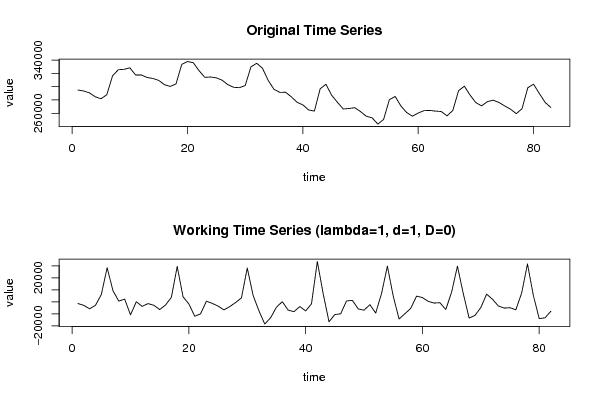
Dataseries X:

Download CSV

Histogram

Boxplots

Summary of computational transaction
Raw Input	view raw input (R code)
Raw Output	view raw output of R engine
Computing time	2 seconds
R Server	'Sir Ronald Aylmer Fisher' @ 193.190.124.24

\begin{tabular}{lllllllll}
\hline
Summary of computational transaction \tabularnewline
Raw Input & view raw input (R code)  \tabularnewline
Raw Output & view raw output of R engine  \tabularnewline
Computing time & 2 seconds \tabularnewline
R Server & 'Sir Ronald Aylmer Fisher' @ 193.190.124.24 \tabularnewline
\hline
\end{tabular}
%Source: https://freestatistics.org/blog/index.php?pk=111170&T=0

[TABLE]
[ROW][C]Summary of computational transaction[/C][/ROW]
[ROW][C]Raw Input[/C][C]view raw input (R code) [/C][/ROW]
[ROW][C]Raw Output[/C][C]view raw output of R engine [/C][/ROW]
[ROW][C]Computing time[/C][C]2 seconds[/C][/ROW]
[ROW][C]R Server[/C][C]'Sir Ronald Aylmer Fisher' @ 193.190.124.24[/C][/ROW]
[/TABLE]
Source: https://freestatistics.org/blog/index.php?pk=111170&T=0

Globally Unique Identifier (entire table): ba.freestatistics.org/blog/index.php?pk=111170&T=0

As an alternative you can also use a QR Code:

The GUIDs for individual cells are displayed in the table below:

Summary of computational transaction
Raw Input	view raw input (R code)
Raw Output	view raw output of R engine
Computing time	2 seconds
R Server	'Sir Ronald Aylmer Fisher' @ 193.190.124.24

Autocorrelation Function
Time lag k	ACF(k)	T-STAT	P-value
1	0.352263	3.1899	0.001008
2	-0.267602	-2.4232	0.008792
3	-0.386269	-3.4978	0.00038
4	-0.251221	-2.2749	0.012761
5	0.043425	0.3932	0.347586
6	0.168653	1.5272	0.065278
7	0.058947	0.5338	0.297466
8	-0.212789	-1.9269	0.028729
9	-0.322664	-2.9218	0.002247
10	-0.22226	-2.0127	0.023717
11	0.326771	2.959	0.002016
12	0.813223	7.364	0
13	0.252059	2.2825	0.012525
14	-0.277386	-2.5118	0.006986
15	-0.367794	-3.3305	0.000651
16	-0.214243	-1.9401	0.027905
17	0.042338	0.3834	0.351214
18	0.142551	1.2909	0.100191
19	0.029283	0.2652	0.395773
20	-0.209071	-1.8932	0.030928
21	-0.271231	-2.4561	0.008079
22	-0.160259	-1.4512	0.075269
23	0.284051	2.5722	0.005954
24	0.651982	5.904	0
25	0.187285	1.6959	0.046845
26	-0.278187	-2.5191	0.006854
27	-0.327097	-2.962	0.001999
28	-0.193466	-1.7519	0.041764
29	0.027326	0.2474	0.402589
30	0.112321	1.0171	0.156047
31	0.014627	0.1325	0.447474
32	-0.185632	-1.681	0.048287
33	-0.206048	-1.8658	0.03282
34	-0.102964	-0.9324	0.176939
35	0.237656	2.1521	0.017166
36	0.515179	4.6651	6e-06
37	0.126618	1.1466	0.127446
38	-0.229015	-2.0738	0.020617
39	-0.241122	-2.1835	0.01593
40	-0.127084	-1.1508	0.12658
41	0.040986	0.3711	0.355744
42	0.089434	0.8099	0.210181
43	0.003574	0.0324	0.487131
44	-0.136943	-1.2401	0.109243
45	-0.142131	-1.2871	0.100848
46	-0.040361	-0.3655	0.357847
47	0.191404	1.7332	0.043406
48	0.357889	3.2408	0.000862

\begin{tabular}{lllllllll}
\hline
Autocorrelation Function \tabularnewline
Time lag k & ACF(k) & T-STAT & P-value \tabularnewline
1 & 0.352263 & 3.1899 & 0.001008 \tabularnewline
2 & -0.267602 & -2.4232 & 0.008792 \tabularnewline
3 & -0.386269 & -3.4978 & 0.00038 \tabularnewline
4 & -0.251221 & -2.2749 & 0.012761 \tabularnewline
5 & 0.043425 & 0.3932 & 0.347586 \tabularnewline
6 & 0.168653 & 1.5272 & 0.065278 \tabularnewline
7 & 0.058947 & 0.5338 & 0.297466 \tabularnewline
8 & -0.212789 & -1.9269 & 0.028729 \tabularnewline
9 & -0.322664 & -2.9218 & 0.002247 \tabularnewline
10 & -0.22226 & -2.0127 & 0.023717 \tabularnewline
11 & 0.326771 & 2.959 & 0.002016 \tabularnewline
12 & 0.813223 & 7.364 & 0 \tabularnewline
13 & 0.252059 & 2.2825 & 0.012525 \tabularnewline
14 & -0.277386 & -2.5118 & 0.006986 \tabularnewline
15 & -0.367794 & -3.3305 & 0.000651 \tabularnewline
16 & -0.214243 & -1.9401 & 0.027905 \tabularnewline
17 & 0.042338 & 0.3834 & 0.351214 \tabularnewline
18 & 0.142551 & 1.2909 & 0.100191 \tabularnewline
19 & 0.029283 & 0.2652 & 0.395773 \tabularnewline
20 & -0.209071 & -1.8932 & 0.030928 \tabularnewline
21 & -0.271231 & -2.4561 & 0.008079 \tabularnewline
22 & -0.160259 & -1.4512 & 0.075269 \tabularnewline
23 & 0.284051 & 2.5722 & 0.005954 \tabularnewline
24 & 0.651982 & 5.904 & 0 \tabularnewline
25 & 0.187285 & 1.6959 & 0.046845 \tabularnewline
26 & -0.278187 & -2.5191 & 0.006854 \tabularnewline
27 & -0.327097 & -2.962 & 0.001999 \tabularnewline
28 & -0.193466 & -1.7519 & 0.041764 \tabularnewline
29 & 0.027326 & 0.2474 & 0.402589 \tabularnewline
30 & 0.112321 & 1.0171 & 0.156047 \tabularnewline
31 & 0.014627 & 0.1325 & 0.447474 \tabularnewline
32 & -0.185632 & -1.681 & 0.048287 \tabularnewline
33 & -0.206048 & -1.8658 & 0.03282 \tabularnewline
34 & -0.102964 & -0.9324 & 0.176939 \tabularnewline
35 & 0.237656 & 2.1521 & 0.017166 \tabularnewline
36 & 0.515179 & 4.6651 & 6e-06 \tabularnewline
37 & 0.126618 & 1.1466 & 0.127446 \tabularnewline
38 & -0.229015 & -2.0738 & 0.020617 \tabularnewline
39 & -0.241122 & -2.1835 & 0.01593 \tabularnewline
40 & -0.127084 & -1.1508 & 0.12658 \tabularnewline
41 & 0.040986 & 0.3711 & 0.355744 \tabularnewline
42 & 0.089434 & 0.8099 & 0.210181 \tabularnewline
43 & 0.003574 & 0.0324 & 0.487131 \tabularnewline
44 & -0.136943 & -1.2401 & 0.109243 \tabularnewline
45 & -0.142131 & -1.2871 & 0.100848 \tabularnewline
46 & -0.040361 & -0.3655 & 0.357847 \tabularnewline
47 & 0.191404 & 1.7332 & 0.043406 \tabularnewline
48 & 0.357889 & 3.2408 & 0.000862 \tabularnewline
\hline
\end{tabular}
%Source: https://freestatistics.org/blog/index.php?pk=111170&T=1

[TABLE]
[ROW][C]Autocorrelation Function[/C][/ROW]
[ROW][C]Time lag k[/C][C]ACF(k)[/C][C]T-STAT[/C][C]P-value[/C][/ROW]
[ROW][C]1[/C][C]0.352263[/C][C]3.1899[/C][C]0.001008[/C][/ROW]
[ROW][C]2[/C][C]-0.267602[/C][C]-2.4232[/C][C]0.008792[/C][/ROW]
[ROW][C]3[/C][C]-0.386269[/C][C]-3.4978[/C][C]0.00038[/C][/ROW]
[ROW][C]4[/C][C]-0.251221[/C][C]-2.2749[/C][C]0.012761[/C][/ROW]
[ROW][C]5[/C][C]0.043425[/C][C]0.3932[/C][C]0.347586[/C][/ROW]
[ROW][C]6[/C][C]0.168653[/C][C]1.5272[/C][C]0.065278[/C][/ROW]
[ROW][C]7[/C][C]0.058947[/C][C]0.5338[/C][C]0.297466[/C][/ROW]
[ROW][C]8[/C][C]-0.212789[/C][C]-1.9269[/C][C]0.028729[/C][/ROW]
[ROW][C]9[/C][C]-0.322664[/C][C]-2.9218[/C][C]0.002247[/C][/ROW]
[ROW][C]10[/C][C]-0.22226[/C][C]-2.0127[/C][C]0.023717[/C][/ROW]
[ROW][C]11[/C][C]0.326771[/C][C]2.959[/C][C]0.002016[/C][/ROW]
[ROW][C]12[/C][C]0.813223[/C][C]7.364[/C][C]0[/C][/ROW]
[ROW][C]13[/C][C]0.252059[/C][C]2.2825[/C][C]0.012525[/C][/ROW]
[ROW][C]14[/C][C]-0.277386[/C][C]-2.5118[/C][C]0.006986[/C][/ROW]
[ROW][C]15[/C][C]-0.367794[/C][C]-3.3305[/C][C]0.000651[/C][/ROW]
[ROW][C]16[/C][C]-0.214243[/C][C]-1.9401[/C][C]0.027905[/C][/ROW]
[ROW][C]17[/C][C]0.042338[/C][C]0.3834[/C][C]0.351214[/C][/ROW]
[ROW][C]18[/C][C]0.142551[/C][C]1.2909[/C][C]0.100191[/C][/ROW]
[ROW][C]19[/C][C]0.029283[/C][C]0.2652[/C][C]0.395773[/C][/ROW]
[ROW][C]20[/C][C]-0.209071[/C][C]-1.8932[/C][C]0.030928[/C][/ROW]
[ROW][C]21[/C][C]-0.271231[/C][C]-2.4561[/C][C]0.008079[/C][/ROW]
[ROW][C]22[/C][C]-0.160259[/C][C]-1.4512[/C][C]0.075269[/C][/ROW]
[ROW][C]23[/C][C]0.284051[/C][C]2.5722[/C][C]0.005954[/C][/ROW]
[ROW][C]24[/C][C]0.651982[/C][C]5.904[/C][C]0[/C][/ROW]
[ROW][C]25[/C][C]0.187285[/C][C]1.6959[/C][C]0.046845[/C][/ROW]
[ROW][C]26[/C][C]-0.278187[/C][C]-2.5191[/C][C]0.006854[/C][/ROW]
[ROW][C]27[/C][C]-0.327097[/C][C]-2.962[/C][C]0.001999[/C][/ROW]
[ROW][C]28[/C][C]-0.193466[/C][C]-1.7519[/C][C]0.041764[/C][/ROW]
[ROW][C]29[/C][C]0.027326[/C][C]0.2474[/C][C]0.402589[/C][/ROW]
[ROW][C]30[/C][C]0.112321[/C][C]1.0171[/C][C]0.156047[/C][/ROW]
[ROW][C]31[/C][C]0.014627[/C][C]0.1325[/C][C]0.447474[/C][/ROW]
[ROW][C]32[/C][C]-0.185632[/C][C]-1.681[/C][C]0.048287[/C][/ROW]
[ROW][C]33[/C][C]-0.206048[/C][C]-1.8658[/C][C]0.03282[/C][/ROW]
[ROW][C]34[/C][C]-0.102964[/C][C]-0.9324[/C][C]0.176939[/C][/ROW]
[ROW][C]35[/C][C]0.237656[/C][C]2.1521[/C][C]0.017166[/C][/ROW]
[ROW][C]36[/C][C]0.515179[/C][C]4.6651[/C][C]6e-06[/C][/ROW]
[ROW][C]37[/C][C]0.126618[/C][C]1.1466[/C][C]0.127446[/C][/ROW]
[ROW][C]38[/C][C]-0.229015[/C][C]-2.0738[/C][C]0.020617[/C][/ROW]
[ROW][C]39[/C][C]-0.241122[/C][C]-2.1835[/C][C]0.01593[/C][/ROW]
[ROW][C]40[/C][C]-0.127084[/C][C]-1.1508[/C][C]0.12658[/C][/ROW]
[ROW][C]41[/C][C]0.040986[/C][C]0.3711[/C][C]0.355744[/C][/ROW]
[ROW][C]42[/C][C]0.089434[/C][C]0.8099[/C][C]0.210181[/C][/ROW]
[ROW][C]43[/C][C]0.003574[/C][C]0.0324[/C][C]0.487131[/C][/ROW]
[ROW][C]44[/C][C]-0.136943[/C][C]-1.2401[/C][C]0.109243[/C][/ROW]
[ROW][C]45[/C][C]-0.142131[/C][C]-1.2871[/C][C]0.100848[/C][/ROW]
[ROW][C]46[/C][C]-0.040361[/C][C]-0.3655[/C][C]0.357847[/C][/ROW]
[ROW][C]47[/C][C]0.191404[/C][C]1.7332[/C][C]0.043406[/C][/ROW]
[ROW][C]48[/C][C]0.357889[/C][C]3.2408[/C][C]0.000862[/C][/ROW]
[/TABLE]
Source: https://freestatistics.org/blog/index.php?pk=111170&T=1

Globally Unique Identifier (entire table): ba.freestatistics.org/blog/index.php?pk=111170&T=1

As an alternative you can also use a QR Code:

The GUIDs for individual cells are displayed in the table below:

Autocorrelation Function
Time lag k	ACF(k)	T-STAT	P-value
1	0.352263	3.1899	0.001008
2	-0.267602	-2.4232	0.008792
3	-0.386269	-3.4978	0.00038
4	-0.251221	-2.2749	0.012761
5	0.043425	0.3932	0.347586
6	0.168653	1.5272	0.065278
7	0.058947	0.5338	0.297466
8	-0.212789	-1.9269	0.028729
9	-0.322664	-2.9218	0.002247
10	-0.22226	-2.0127	0.023717
11	0.326771	2.959	0.002016
12	0.813223	7.364	0
13	0.252059	2.2825	0.012525
14	-0.277386	-2.5118	0.006986
15	-0.367794	-3.3305	0.000651
16	-0.214243	-1.9401	0.027905
17	0.042338	0.3834	0.351214
18	0.142551	1.2909	0.100191
19	0.029283	0.2652	0.395773
20	-0.209071	-1.8932	0.030928
21	-0.271231	-2.4561	0.008079
22	-0.160259	-1.4512	0.075269
23	0.284051	2.5722	0.005954
24	0.651982	5.904	0
25	0.187285	1.6959	0.046845
26	-0.278187	-2.5191	0.006854
27	-0.327097	-2.962	0.001999
28	-0.193466	-1.7519	0.041764
29	0.027326	0.2474	0.402589
30	0.112321	1.0171	0.156047
31	0.014627	0.1325	0.447474
32	-0.185632	-1.681	0.048287
33	-0.206048	-1.8658	0.03282
34	-0.102964	-0.9324	0.176939
35	0.237656	2.1521	0.017166
36	0.515179	4.6651	6e-06
37	0.126618	1.1466	0.127446
38	-0.229015	-2.0738	0.020617
39	-0.241122	-2.1835	0.01593
40	-0.127084	-1.1508	0.12658
41	0.040986	0.3711	0.355744
42	0.089434	0.8099	0.210181
43	0.003574	0.0324	0.487131
44	-0.136943	-1.2401	0.109243
45	-0.142131	-1.2871	0.100848
46	-0.040361	-0.3655	0.357847
47	0.191404	1.7332	0.043406
48	0.357889	3.2408	0.000862

Partial Autocorrelation Function
Time lag k	PACF(k)	T-STAT	P-value
1	0.352263	3.1899	0.001008
2	-0.447182	-4.0494	5.8e-05
3	-0.131748	-1.193	0.11815
4	-0.192199	-1.7404	0.042767
5	0.046699	0.4229	0.336746
6	-0.069443	-0.6288	0.265604
7	-0.076037	-0.6885	0.246527
8	-0.286116	-2.5909	0.005664
9	-0.220249	-1.9944	0.024713
10	-0.332467	-3.0106	0.001732
11	0.348589	3.1566	0.001117
12	0.599007	5.4242	0
13	-0.276509	-2.5039	0.007133
14	0.120913	1.0949	0.13838
15	0.054662	0.495	0.310967
16	0.051896	0.4699	0.319824
17	-0.068724	-0.6223	0.267728
18	-0.058183	-0.5269	0.299853
19	-0.084696	-0.767	0.222654
20	-0.075835	-0.6867	0.247099
21	-0.019913	-0.1803	0.428673
22	-0.021639	-0.1959	0.422568
23	-0.163966	-1.4848	0.070719
24	0.002095	0.019	0.492454
25	-0.002935	-0.0266	0.489431
26	-0.090455	-0.8191	0.20755
27	0.025478	0.2307	0.409057
28	-0.147522	-1.3359	0.092645
29	-0.027748	-0.2513	0.401118
30	-0.092143	-0.8344	0.203243
31	-0.014585	-0.1321	0.447625
32	-0.085003	-0.7697	0.221834
33	-0.021676	-0.1963	0.422435
34	-0.074022	-0.6703	0.252276
35	-0.061623	-0.558	0.289175
36	-0.090574	-0.8202	0.207244
37	-0.064201	-0.5814	0.281295
38	0.046783	0.4236	0.336471
39	-0.007975	-0.0722	0.471302
40	0.054284	0.4916	0.312172
41	-0.002538	-0.023	0.49086
42	0.016271	0.1473	0.441612
43	0.01331	0.1205	0.452182
44	0.106008	0.9599	0.169953
45	-0.064689	-0.5858	0.279815
46	0.100369	0.9089	0.183037
47	-0.123284	-1.1164	0.133758
48	-0.098939	-0.8959	0.186456

\begin{tabular}{lllllllll}
\hline
Partial Autocorrelation Function \tabularnewline
Time lag k & PACF(k) & T-STAT & P-value \tabularnewline
1 & 0.352263 & 3.1899 & 0.001008 \tabularnewline
2 & -0.447182 & -4.0494 & 5.8e-05 \tabularnewline
3 & -0.131748 & -1.193 & 0.11815 \tabularnewline
4 & -0.192199 & -1.7404 & 0.042767 \tabularnewline
5 & 0.046699 & 0.4229 & 0.336746 \tabularnewline
6 & -0.069443 & -0.6288 & 0.265604 \tabularnewline
7 & -0.076037 & -0.6885 & 0.246527 \tabularnewline
8 & -0.286116 & -2.5909 & 0.005664 \tabularnewline
9 & -0.220249 & -1.9944 & 0.024713 \tabularnewline
10 & -0.332467 & -3.0106 & 0.001732 \tabularnewline
11 & 0.348589 & 3.1566 & 0.001117 \tabularnewline
12 & 0.599007 & 5.4242 & 0 \tabularnewline
13 & -0.276509 & -2.5039 & 0.007133 \tabularnewline
14 & 0.120913 & 1.0949 & 0.13838 \tabularnewline
15 & 0.054662 & 0.495 & 0.310967 \tabularnewline
16 & 0.051896 & 0.4699 & 0.319824 \tabularnewline
17 & -0.068724 & -0.6223 & 0.267728 \tabularnewline
18 & -0.058183 & -0.5269 & 0.299853 \tabularnewline
19 & -0.084696 & -0.767 & 0.222654 \tabularnewline
20 & -0.075835 & -0.6867 & 0.247099 \tabularnewline
21 & -0.019913 & -0.1803 & 0.428673 \tabularnewline
22 & -0.021639 & -0.1959 & 0.422568 \tabularnewline
23 & -0.163966 & -1.4848 & 0.070719 \tabularnewline
24 & 0.002095 & 0.019 & 0.492454 \tabularnewline
25 & -0.002935 & -0.0266 & 0.489431 \tabularnewline
26 & -0.090455 & -0.8191 & 0.20755 \tabularnewline
27 & 0.025478 & 0.2307 & 0.409057 \tabularnewline
28 & -0.147522 & -1.3359 & 0.092645 \tabularnewline
29 & -0.027748 & -0.2513 & 0.401118 \tabularnewline
30 & -0.092143 & -0.8344 & 0.203243 \tabularnewline
31 & -0.014585 & -0.1321 & 0.447625 \tabularnewline
32 & -0.085003 & -0.7697 & 0.221834 \tabularnewline
33 & -0.021676 & -0.1963 & 0.422435 \tabularnewline
34 & -0.074022 & -0.6703 & 0.252276 \tabularnewline
35 & -0.061623 & -0.558 & 0.289175 \tabularnewline
36 & -0.090574 & -0.8202 & 0.207244 \tabularnewline
37 & -0.064201 & -0.5814 & 0.281295 \tabularnewline
38 & 0.046783 & 0.4236 & 0.336471 \tabularnewline
39 & -0.007975 & -0.0722 & 0.471302 \tabularnewline
40 & 0.054284 & 0.4916 & 0.312172 \tabularnewline
41 & -0.002538 & -0.023 & 0.49086 \tabularnewline
42 & 0.016271 & 0.1473 & 0.441612 \tabularnewline
43 & 0.01331 & 0.1205 & 0.452182 \tabularnewline
44 & 0.106008 & 0.9599 & 0.169953 \tabularnewline
45 & -0.064689 & -0.5858 & 0.279815 \tabularnewline
46 & 0.100369 & 0.9089 & 0.183037 \tabularnewline
47 & -0.123284 & -1.1164 & 0.133758 \tabularnewline
48 & -0.098939 & -0.8959 & 0.186456 \tabularnewline
\hline
\end{tabular}
%Source: https://freestatistics.org/blog/index.php?pk=111170&T=2

[TABLE]
[ROW][C]Partial Autocorrelation Function[/C][/ROW]
[ROW][C]Time lag k[/C][C]PACF(k)[/C][C]T-STAT[/C][C]P-value[/C][/ROW]
[ROW][C]1[/C][C]0.352263[/C][C]3.1899[/C][C]0.001008[/C][/ROW]
[ROW][C]2[/C][C]-0.447182[/C][C]-4.0494[/C][C]5.8e-05[/C][/ROW]
[ROW][C]3[/C][C]-0.131748[/C][C]-1.193[/C][C]0.11815[/C][/ROW]
[ROW][C]4[/C][C]-0.192199[/C][C]-1.7404[/C][C]0.042767[/C][/ROW]
[ROW][C]5[/C][C]0.046699[/C][C]0.4229[/C][C]0.336746[/C][/ROW]
[ROW][C]6[/C][C]-0.069443[/C][C]-0.6288[/C][C]0.265604[/C][/ROW]
[ROW][C]7[/C][C]-0.076037[/C][C]-0.6885[/C][C]0.246527[/C][/ROW]
[ROW][C]8[/C][C]-0.286116[/C][C]-2.5909[/C][C]0.005664[/C][/ROW]
[ROW][C]9[/C][C]-0.220249[/C][C]-1.9944[/C][C]0.024713[/C][/ROW]
[ROW][C]10[/C][C]-0.332467[/C][C]-3.0106[/C][C]0.001732[/C][/ROW]
[ROW][C]11[/C][C]0.348589[/C][C]3.1566[/C][C]0.001117[/C][/ROW]
[ROW][C]12[/C][C]0.599007[/C][C]5.4242[/C][C]0[/C][/ROW]
[ROW][C]13[/C][C]-0.276509[/C][C]-2.5039[/C][C]0.007133[/C][/ROW]
[ROW][C]14[/C][C]0.120913[/C][C]1.0949[/C][C]0.13838[/C][/ROW]
[ROW][C]15[/C][C]0.054662[/C][C]0.495[/C][C]0.310967[/C][/ROW]
[ROW][C]16[/C][C]0.051896[/C][C]0.4699[/C][C]0.319824[/C][/ROW]
[ROW][C]17[/C][C]-0.068724[/C][C]-0.6223[/C][C]0.267728[/C][/ROW]
[ROW][C]18[/C][C]-0.058183[/C][C]-0.5269[/C][C]0.299853[/C][/ROW]
[ROW][C]19[/C][C]-0.084696[/C][C]-0.767[/C][C]0.222654[/C][/ROW]
[ROW][C]20[/C][C]-0.075835[/C][C]-0.6867[/C][C]0.247099[/C][/ROW]
[ROW][C]21[/C][C]-0.019913[/C][C]-0.1803[/C][C]0.428673[/C][/ROW]
[ROW][C]22[/C][C]-0.021639[/C][C]-0.1959[/C][C]0.422568[/C][/ROW]
[ROW][C]23[/C][C]-0.163966[/C][C]-1.4848[/C][C]0.070719[/C][/ROW]
[ROW][C]24[/C][C]0.002095[/C][C]0.019[/C][C]0.492454[/C][/ROW]
[ROW][C]25[/C][C]-0.002935[/C][C]-0.0266[/C][C]0.489431[/C][/ROW]
[ROW][C]26[/C][C]-0.090455[/C][C]-0.8191[/C][C]0.20755[/C][/ROW]
[ROW][C]27[/C][C]0.025478[/C][C]0.2307[/C][C]0.409057[/C][/ROW]
[ROW][C]28[/C][C]-0.147522[/C][C]-1.3359[/C][C]0.092645[/C][/ROW]
[ROW][C]29[/C][C]-0.027748[/C][C]-0.2513[/C][C]0.401118[/C][/ROW]
[ROW][C]30[/C][C]-0.092143[/C][C]-0.8344[/C][C]0.203243[/C][/ROW]
[ROW][C]31[/C][C]-0.014585[/C][C]-0.1321[/C][C]0.447625[/C][/ROW]
[ROW][C]32[/C][C]-0.085003[/C][C]-0.7697[/C][C]0.221834[/C][/ROW]
[ROW][C]33[/C][C]-0.021676[/C][C]-0.1963[/C][C]0.422435[/C][/ROW]
[ROW][C]34[/C][C]-0.074022[/C][C]-0.6703[/C][C]0.252276[/C][/ROW]
[ROW][C]35[/C][C]-0.061623[/C][C]-0.558[/C][C]0.289175[/C][/ROW]
[ROW][C]36[/C][C]-0.090574[/C][C]-0.8202[/C][C]0.207244[/C][/ROW]
[ROW][C]37[/C][C]-0.064201[/C][C]-0.5814[/C][C]0.281295[/C][/ROW]
[ROW][C]38[/C][C]0.046783[/C][C]0.4236[/C][C]0.336471[/C][/ROW]
[ROW][C]39[/C][C]-0.007975[/C][C]-0.0722[/C][C]0.471302[/C][/ROW]
[ROW][C]40[/C][C]0.054284[/C][C]0.4916[/C][C]0.312172[/C][/ROW]
[ROW][C]41[/C][C]-0.002538[/C][C]-0.023[/C][C]0.49086[/C][/ROW]
[ROW][C]42[/C][C]0.016271[/C][C]0.1473[/C][C]0.441612[/C][/ROW]
[ROW][C]43[/C][C]0.01331[/C][C]0.1205[/C][C]0.452182[/C][/ROW]
[ROW][C]44[/C][C]0.106008[/C][C]0.9599[/C][C]0.169953[/C][/ROW]
[ROW][C]45[/C][C]-0.064689[/C][C]-0.5858[/C][C]0.279815[/C][/ROW]
[ROW][C]46[/C][C]0.100369[/C][C]0.9089[/C][C]0.183037[/C][/ROW]
[ROW][C]47[/C][C]-0.123284[/C][C]-1.1164[/C][C]0.133758[/C][/ROW]
[ROW][C]48[/C][C]-0.098939[/C][C]-0.8959[/C][C]0.186456[/C][/ROW]
[/TABLE]
Source: https://freestatistics.org/blog/index.php?pk=111170&T=2

Globally Unique Identifier (entire table): ba.freestatistics.org/blog/index.php?pk=111170&T=2

As an alternative you can also use a QR Code:

The GUIDs for individual cells are displayed in the table below:

Partial Autocorrelation Function
Time lag k	PACF(k)	T-STAT	P-value
1	0.352263	3.1899	0.001008
2	-0.447182	-4.0494	5.8e-05
3	-0.131748	-1.193	0.11815
4	-0.192199	-1.7404	0.042767
5	0.046699	0.4229	0.336746
6	-0.069443	-0.6288	0.265604
7	-0.076037	-0.6885	0.246527
8	-0.286116	-2.5909	0.005664
9	-0.220249	-1.9944	0.024713
10	-0.332467	-3.0106	0.001732
11	0.348589	3.1566	0.001117
12	0.599007	5.4242	0
13	-0.276509	-2.5039	0.007133
14	0.120913	1.0949	0.13838
15	0.054662	0.495	0.310967
16	0.051896	0.4699	0.319824
17	-0.068724	-0.6223	0.267728
18	-0.058183	-0.5269	0.299853
19	-0.084696	-0.767	0.222654
20	-0.075835	-0.6867	0.247099
21	-0.019913	-0.1803	0.428673
22	-0.021639	-0.1959	0.422568
23	-0.163966	-1.4848	0.070719
24	0.002095	0.019	0.492454
25	-0.002935	-0.0266	0.489431
26	-0.090455	-0.8191	0.20755
27	0.025478	0.2307	0.409057
28	-0.147522	-1.3359	0.092645
29	-0.027748	-0.2513	0.401118
30	-0.092143	-0.8344	0.203243
31	-0.014585	-0.1321	0.447625
32	-0.085003	-0.7697	0.221834
33	-0.021676	-0.1963	0.422435
34	-0.074022	-0.6703	0.252276
35	-0.061623	-0.558	0.289175
36	-0.090574	-0.8202	0.207244
37	-0.064201	-0.5814	0.281295
38	0.046783	0.4236	0.336471
39	-0.007975	-0.0722	0.471302
40	0.054284	0.4916	0.312172
41	-0.002538	-0.023	0.49086
42	0.016271	0.1473	0.441612
43	0.01331	0.1205	0.452182
44	0.106008	0.9599	0.169953
45	-0.064689	-0.5858	0.279815
46	0.100369	0.9089	0.183037
47	-0.123284	-1.1164	0.133758
48	-0.098939	-0.8959	0.186456

Figure 1

PNG link

Postscript link

PDF link

Figure 2

PNG link

Postscript link

PDF link

Figure 3

PNG link

Postscript link

PDF link

Parameters (Session):

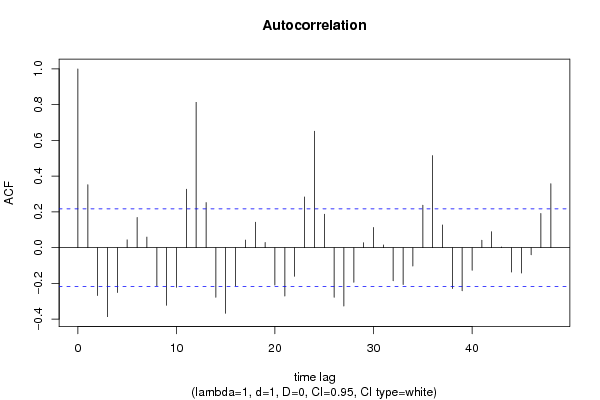
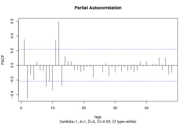
par1 = 48 ; par2 = 1 ; par3 = 1 ; par4 = 0 ; par5 = 12 ; par6 = White Noise ; par7 = 0.95 ;

Parameters (R input):

par1 = 48 ; par2 = 1 ; par3 = 1 ; par4 = 0 ; par5 = 12 ; par6 = White Noise ; par7 = 0.95 ; par8 = ;

R code (references can be found in the software module):

if (par1 == 'Default') {
par1 = 10*log10(length(x))
} else {
par1 <- as.numeric(par1)
}
par2 <- as.numeric(par2)
par3 <- as.numeric(par3)
par4 <- as.numeric(par4)
par5 <- as.numeric(par5)
if (par6 == 'White Noise') par6 <- 'white' else par6 <- 'ma'
par7 <- as.numeric(par7)
if (par8 != '') par8 <- as.numeric(par8)
ox <- x
if (par8 == '') {
if (par2 == 0) {
x <- log(x)
} else {
x <- (x ^ par2 - 1) / par2
}
} else {
x <- log(x,base=par8)
}
if (par3 > 0) x <- diff(x,lag=1,difference=par3)
if (par4 > 0) x <- diff(x,lag=par5,difference=par4)
bitmap(file='picts.png')
op <- par(mfrow=c(2,1))
plot(ox,type='l',main='Original Time Series',xlab='time',ylab='value')
if (par8=='') {
mytitle <- paste('Working Time Series (lambda=',par2,', d=',par3,', D=',par4,')',sep='')
mysub <- paste('(lambda=',par2,', d=',par3,', D=',par4,', CI=', par7, ', CI type=',par6,')',sep='')
} else {
mytitle <- paste('Working Time Series (base=',par8,', d=',par3,', D=',par4,')',sep='')
mysub <- paste('(base=',par8,', d=',par3,', D=',par4,', CI=', par7, ', CI type=',par6,')',sep='')
}
plot(x,type='l', main=mytitle,xlab='time',ylab='value')
par(op)
dev.off()
bitmap(file='pic1.png')
racf <- acf(x, par1, main='Autocorrelation', xlab='time lag', ylab='ACF', ci.type=par6, ci=par7, sub=mysub)
dev.off()
bitmap(file='pic2.png')
rpacf <- pacf(x,par1,main='Partial Autocorrelation',xlab='lags',ylab='PACF',sub=mysub)
dev.off()
(myacf <- c(racf$acf))
(mypacf <- c(rpacf$acf))
lengthx <- length(x)
sqrtn <- sqrt(lengthx)
load(file='createtable')
a<-table.start()
a<-table.row.start(a)
a<-table.element(a,'Autocorrelation Function',4,TRUE)
a<-table.row.end(a)
a<-table.row.start(a)
a<-table.element(a,'Time lag k',header=TRUE)
a<-table.element(a,hyperlink('basics.htm','ACF(k)','click here for more information about the Autocorrelation Function'),header=TRUE)
a<-table.element(a,'T-STAT',header=TRUE)
a<-table.element(a,'P-value',header=TRUE)
a<-table.row.end(a)
for (i in 2:(par1+1)) {
a<-table.row.start(a)
a<-table.element(a,i-1,header=TRUE)
a<-table.element(a,round(myacf[i],6))
mytstat <- myacf[i]*sqrtn
a<-table.element(a,round(mytstat,4))
a<-table.element(a,round(1-pt(abs(mytstat),lengthx),6))
a<-table.row.end(a)
}
a<-table.end(a)
table.save(a,file='mytable.tab')
a<-table.start()
a<-table.row.start(a)
a<-table.element(a,'Partial Autocorrelation Function',4,TRUE)
a<-table.row.end(a)
a<-table.row.start(a)
a<-table.element(a,'Time lag k',header=TRUE)
a<-table.element(a,hyperlink('basics.htm','PACF(k)','click here for more information about the Partial Autocorrelation Function'),header=TRUE)
a<-table.element(a,'T-STAT',header=TRUE)
a<-table.element(a,'P-value',header=TRUE)
a<-table.row.end(a)
for (i in 1:par1) {
a<-table.row.start(a)
a<-table.element(a,i,header=TRUE)
a<-table.element(a,round(mypacf[i],6))
mytstat <- mypacf[i]*sqrtn
a<-table.element(a,round(mytstat,4))
a<-table.element(a,round(1-pt(abs(mytstat),lengthx),6))
a<-table.row.end(a)
}
a<-table.end(a)
table.save(a,file='mytable1.tab')

Free Statistics

Description of Statistical Computation

Tree of Dependent Computations

Dataset

Tables (Output of Computation)

Figures (Output of Computation)

Input Parameters & R Code