Repository of Reproducible Computations

Free Statistics

of Irreproducible Research!

Author's title

Author

*The author of this computation has been verified*

R Software Module

rwasp_autocorrelation.wasp

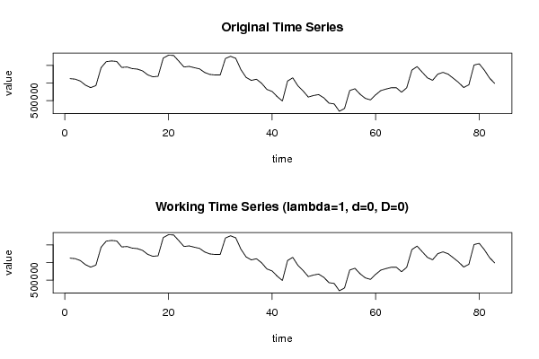
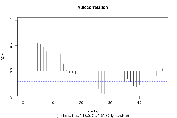
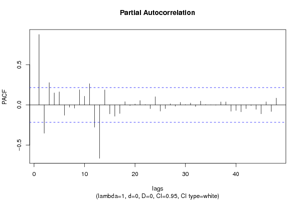
Title produced by software

(Partial) Autocorrelation Function

Date of computation

Sun, 19 Dec 2010 14:45:15 +0000

Cite this page as follows

Statistical Computations at FreeStatistics.org, Office for Research Development and Education, URL https://freestatistics.org/blog/index.php?v=date/2010/Dec/19/t1292769811iqpi65o04e7fw1t.htm/, Retrieved Tue, 30 Apr 2024 04:25:44 +0000

Statistical Computations at FreeStatistics.org, Office for Research Development and Education, URL https://freestatistics.org/blog/index.php?pk=112447, Retrieved Tue, 30 Apr 2024 04:25:44 +0000

QR Codes:

Paste this QR Code to cite your computation.

Original text written by user:

IsPrivate?

No (this computation is public)

User-defined keywords

Estimated Impact

173

Family? (F = Feedback message, R = changed R code, M = changed R Module, P = changed Parameters, D = changed Data)

-     [Multiple Regression] [Q1 The Seatbeltlaw] [2007-11-14 19:27:43] [8cd6641b921d30ebe00b648d1481bba0]
- RMPD  [Multiple Regression] [Seatbelt] [2009-11-12 13:54:52] [b98453cac15ba1066b407e146608df68]
-    D    [Multiple Regression] [WS7] [2009-11-18 17:01:04] [8b1aef4e7013bd33fbc2a5833375c5f5]
-   PD      [Multiple Regression] [WS7(2)] [2009-11-20 19:01:46] [7d268329e554b8694908ba13e6e6f258]
-   P         [Multiple Regression] [WS7(3)] [2009-11-21 10:22:47] [7d268329e554b8694908ba13e6e6f258]
-   PD          [Multiple Regression] [WS7(4)] [2009-11-21 10:55:20] [7d268329e554b8694908ba13e6e6f258]
- RMPD            [Univariate Data Series] [Niet-werkende wer...] [2009-11-25 19:16:52] [9717cb857c153ca3061376906953b329]
-   PD              [Univariate Data Series] [] [2010-12-16 17:58:43] [bcc4ad4a6c0f95d5b548de29638ac6c2]
-   PD                [Univariate Data Series] [] [2010-12-19 14:40:10] [bcc4ad4a6c0f95d5b548de29638ac6c2]
- RMP                     [(Partial) Autocorrelation Function] [] [2010-12-19 14:45:15] [4e3652732e77bb1a104cdb5f8d687d01] [Current]

Feedback Forum

Post a new message

Dataseries X:

Download CSV

Histogram

Boxplots

Summary of computational transaction
Raw Input	view raw input (R code)
Raw Output	view raw output of R engine
Computing time	4 seconds
R Server	'Gwilym Jenkins' @ 72.249.127.135

\begin{tabular}{lllllllll}
\hline
Summary of computational transaction \tabularnewline
Raw Input & view raw input (R code)  \tabularnewline
Raw Output & view raw output of R engine  \tabularnewline
Computing time & 4 seconds \tabularnewline
R Server & 'Gwilym Jenkins' @ 72.249.127.135 \tabularnewline
\hline
\end{tabular}
%Source: https://freestatistics.org/blog/index.php?pk=112447&T=0

[TABLE]
[ROW][C]Summary of computational transaction[/C][/ROW]
[ROW][C]Raw Input[/C][C]view raw input (R code) [/C][/ROW]
[ROW][C]Raw Output[/C][C]view raw output of R engine [/C][/ROW]
[ROW][C]Computing time[/C][C]4 seconds[/C][/ROW]
[ROW][C]R Server[/C][C]'Gwilym Jenkins' @ 72.249.127.135[/C][/ROW]
[/TABLE]
Source: https://freestatistics.org/blog/index.php?pk=112447&T=0

Globally Unique Identifier (entire table): ba.freestatistics.org/blog/index.php?pk=112447&T=0

As an alternative you can also use a QR Code:

The GUIDs for individual cells are displayed in the table below:

Summary of computational transaction
Raw Input	view raw input (R code)
Raw Output	view raw output of R engine
Computing time	4 seconds
R Server	'Gwilym Jenkins' @ 72.249.127.135

Autocorrelation Function
Time lag k	ACF(k)	T-STAT	P-value
1	0.875848	7.9794	0
2	0.685036	6.241	0
3	0.559328	5.0957	1e-06
4	0.521711	4.753	4e-06
5	0.542834	4.9455	2e-06
6	0.534856	4.8728	3e-06
7	0.4708	4.2892	2.4e-05
8	0.381561	3.4762	0.000406
9	0.34238	3.1192	0.001247
10	0.376912	3.4338	0.000466
11	0.469864	4.2807	2.5e-05
12	0.499917	4.5545	9e-06
13	0.337581	3.0755	0.001423
14	0.136657	1.245	0.108317
15	0.003404	0.031	0.487666
16	-0.046101	-0.42	0.337785
17	-0.046344	-0.4222	0.336982
18	-0.072859	-0.6638	0.254338
19	-0.143016	-1.3029	0.098099
20	-0.223482	-2.036	0.022469
21	-0.251434	-2.2907	0.012259
22	-0.213926	-1.949	0.027339
23	-0.130603	-1.1898	0.118749
24	-0.101316	-0.923	0.179332
25	-0.223818	-2.0391	0.022312
26	-0.36997	-3.3706	0.00057
27	-0.44924	-4.0928	4.9e-05
28	-0.452916	-4.1263	4.4e-05
29	-0.411966	-3.7532	0.000161
30	-0.393489	-3.5849	0.000284
31	-0.411144	-3.7457	0.000166
32	-0.434528	-3.9587	7.9e-05
33	-0.409453	-3.7303	0.000174
34	-0.331869	-3.0235	0.001662
35	-0.221841	-2.0211	0.023248
36	-0.161861	-1.4746	0.072048
37	-0.224681	-2.0469	0.021914
38	-0.299603	-2.7295	0.003871
39	-0.321097	-2.9253	0.002218
40	-0.289141	-2.6342	0.00503
41	-0.232622	-2.1193	0.018527
42	-0.20376	-1.8563	0.033476
43	-0.203822	-1.8569	0.033436
44	-0.205729	-1.8743	0.032205
45	-0.171267	-1.5603	0.061245
46	-0.097315	-0.8866	0.188932
47	-0.008087	-0.0737	0.470722
48	0.038312	0.349	0.363972

\begin{tabular}{lllllllll}
\hline
Autocorrelation Function \tabularnewline
Time lag k & ACF(k) & T-STAT & P-value \tabularnewline
1 & 0.875848 & 7.9794 & 0 \tabularnewline
2 & 0.685036 & 6.241 & 0 \tabularnewline
3 & 0.559328 & 5.0957 & 1e-06 \tabularnewline
4 & 0.521711 & 4.753 & 4e-06 \tabularnewline
5 & 0.542834 & 4.9455 & 2e-06 \tabularnewline
6 & 0.534856 & 4.8728 & 3e-06 \tabularnewline
7 & 0.4708 & 4.2892 & 2.4e-05 \tabularnewline
8 & 0.381561 & 3.4762 & 0.000406 \tabularnewline
9 & 0.34238 & 3.1192 & 0.001247 \tabularnewline
10 & 0.376912 & 3.4338 & 0.000466 \tabularnewline
11 & 0.469864 & 4.2807 & 2.5e-05 \tabularnewline
12 & 0.499917 & 4.5545 & 9e-06 \tabularnewline
13 & 0.337581 & 3.0755 & 0.001423 \tabularnewline
14 & 0.136657 & 1.245 & 0.108317 \tabularnewline
15 & 0.003404 & 0.031 & 0.487666 \tabularnewline
16 & -0.046101 & -0.42 & 0.337785 \tabularnewline
17 & -0.046344 & -0.4222 & 0.336982 \tabularnewline
18 & -0.072859 & -0.6638 & 0.254338 \tabularnewline
19 & -0.143016 & -1.3029 & 0.098099 \tabularnewline
20 & -0.223482 & -2.036 & 0.022469 \tabularnewline
21 & -0.251434 & -2.2907 & 0.012259 \tabularnewline
22 & -0.213926 & -1.949 & 0.027339 \tabularnewline
23 & -0.130603 & -1.1898 & 0.118749 \tabularnewline
24 & -0.101316 & -0.923 & 0.179332 \tabularnewline
25 & -0.223818 & -2.0391 & 0.022312 \tabularnewline
26 & -0.36997 & -3.3706 & 0.00057 \tabularnewline
27 & -0.44924 & -4.0928 & 4.9e-05 \tabularnewline
28 & -0.452916 & -4.1263 & 4.4e-05 \tabularnewline
29 & -0.411966 & -3.7532 & 0.000161 \tabularnewline
30 & -0.393489 & -3.5849 & 0.000284 \tabularnewline
31 & -0.411144 & -3.7457 & 0.000166 \tabularnewline
32 & -0.434528 & -3.9587 & 7.9e-05 \tabularnewline
33 & -0.409453 & -3.7303 & 0.000174 \tabularnewline
34 & -0.331869 & -3.0235 & 0.001662 \tabularnewline
35 & -0.221841 & -2.0211 & 0.023248 \tabularnewline
36 & -0.161861 & -1.4746 & 0.072048 \tabularnewline
37 & -0.224681 & -2.0469 & 0.021914 \tabularnewline
38 & -0.299603 & -2.7295 & 0.003871 \tabularnewline
39 & -0.321097 & -2.9253 & 0.002218 \tabularnewline
40 & -0.289141 & -2.6342 & 0.00503 \tabularnewline
41 & -0.232622 & -2.1193 & 0.018527 \tabularnewline
42 & -0.20376 & -1.8563 & 0.033476 \tabularnewline
43 & -0.203822 & -1.8569 & 0.033436 \tabularnewline
44 & -0.205729 & -1.8743 & 0.032205 \tabularnewline
45 & -0.171267 & -1.5603 & 0.061245 \tabularnewline
46 & -0.097315 & -0.8866 & 0.188932 \tabularnewline
47 & -0.008087 & -0.0737 & 0.470722 \tabularnewline
48 & 0.038312 & 0.349 & 0.363972 \tabularnewline
\hline
\end{tabular}
%Source: https://freestatistics.org/blog/index.php?pk=112447&T=1

[TABLE]
[ROW][C]Autocorrelation Function[/C][/ROW]
[ROW][C]Time lag k[/C][C]ACF(k)[/C][C]T-STAT[/C][C]P-value[/C][/ROW]
[ROW][C]1[/C][C]0.875848[/C][C]7.9794[/C][C]0[/C][/ROW]
[ROW][C]2[/C][C]0.685036[/C][C]6.241[/C][C]0[/C][/ROW]
[ROW][C]3[/C][C]0.559328[/C][C]5.0957[/C][C]1e-06[/C][/ROW]
[ROW][C]4[/C][C]0.521711[/C][C]4.753[/C][C]4e-06[/C][/ROW]
[ROW][C]5[/C][C]0.542834[/C][C]4.9455[/C][C]2e-06[/C][/ROW]
[ROW][C]6[/C][C]0.534856[/C][C]4.8728[/C][C]3e-06[/C][/ROW]
[ROW][C]7[/C][C]0.4708[/C][C]4.2892[/C][C]2.4e-05[/C][/ROW]
[ROW][C]8[/C][C]0.381561[/C][C]3.4762[/C][C]0.000406[/C][/ROW]
[ROW][C]9[/C][C]0.34238[/C][C]3.1192[/C][C]0.001247[/C][/ROW]
[ROW][C]10[/C][C]0.376912[/C][C]3.4338[/C][C]0.000466[/C][/ROW]
[ROW][C]11[/C][C]0.469864[/C][C]4.2807[/C][C]2.5e-05[/C][/ROW]
[ROW][C]12[/C][C]0.499917[/C][C]4.5545[/C][C]9e-06[/C][/ROW]
[ROW][C]13[/C][C]0.337581[/C][C]3.0755[/C][C]0.001423[/C][/ROW]
[ROW][C]14[/C][C]0.136657[/C][C]1.245[/C][C]0.108317[/C][/ROW]
[ROW][C]15[/C][C]0.003404[/C][C]0.031[/C][C]0.487666[/C][/ROW]
[ROW][C]16[/C][C]-0.046101[/C][C]-0.42[/C][C]0.337785[/C][/ROW]
[ROW][C]17[/C][C]-0.046344[/C][C]-0.4222[/C][C]0.336982[/C][/ROW]
[ROW][C]18[/C][C]-0.072859[/C][C]-0.6638[/C][C]0.254338[/C][/ROW]
[ROW][C]19[/C][C]-0.143016[/C][C]-1.3029[/C][C]0.098099[/C][/ROW]
[ROW][C]20[/C][C]-0.223482[/C][C]-2.036[/C][C]0.022469[/C][/ROW]
[ROW][C]21[/C][C]-0.251434[/C][C]-2.2907[/C][C]0.012259[/C][/ROW]
[ROW][C]22[/C][C]-0.213926[/C][C]-1.949[/C][C]0.027339[/C][/ROW]
[ROW][C]23[/C][C]-0.130603[/C][C]-1.1898[/C][C]0.118749[/C][/ROW]
[ROW][C]24[/C][C]-0.101316[/C][C]-0.923[/C][C]0.179332[/C][/ROW]
[ROW][C]25[/C][C]-0.223818[/C][C]-2.0391[/C][C]0.022312[/C][/ROW]
[ROW][C]26[/C][C]-0.36997[/C][C]-3.3706[/C][C]0.00057[/C][/ROW]
[ROW][C]27[/C][C]-0.44924[/C][C]-4.0928[/C][C]4.9e-05[/C][/ROW]
[ROW][C]28[/C][C]-0.452916[/C][C]-4.1263[/C][C]4.4e-05[/C][/ROW]
[ROW][C]29[/C][C]-0.411966[/C][C]-3.7532[/C][C]0.000161[/C][/ROW]
[ROW][C]30[/C][C]-0.393489[/C][C]-3.5849[/C][C]0.000284[/C][/ROW]
[ROW][C]31[/C][C]-0.411144[/C][C]-3.7457[/C][C]0.000166[/C][/ROW]
[ROW][C]32[/C][C]-0.434528[/C][C]-3.9587[/C][C]7.9e-05[/C][/ROW]
[ROW][C]33[/C][C]-0.409453[/C][C]-3.7303[/C][C]0.000174[/C][/ROW]
[ROW][C]34[/C][C]-0.331869[/C][C]-3.0235[/C][C]0.001662[/C][/ROW]
[ROW][C]35[/C][C]-0.221841[/C][C]-2.0211[/C][C]0.023248[/C][/ROW]
[ROW][C]36[/C][C]-0.161861[/C][C]-1.4746[/C][C]0.072048[/C][/ROW]
[ROW][C]37[/C][C]-0.224681[/C][C]-2.0469[/C][C]0.021914[/C][/ROW]
[ROW][C]38[/C][C]-0.299603[/C][C]-2.7295[/C][C]0.003871[/C][/ROW]
[ROW][C]39[/C][C]-0.321097[/C][C]-2.9253[/C][C]0.002218[/C][/ROW]
[ROW][C]40[/C][C]-0.289141[/C][C]-2.6342[/C][C]0.00503[/C][/ROW]
[ROW][C]41[/C][C]-0.232622[/C][C]-2.1193[/C][C]0.018527[/C][/ROW]
[ROW][C]42[/C][C]-0.20376[/C][C]-1.8563[/C][C]0.033476[/C][/ROW]
[ROW][C]43[/C][C]-0.203822[/C][C]-1.8569[/C][C]0.033436[/C][/ROW]
[ROW][C]44[/C][C]-0.205729[/C][C]-1.8743[/C][C]0.032205[/C][/ROW]
[ROW][C]45[/C][C]-0.171267[/C][C]-1.5603[/C][C]0.061245[/C][/ROW]
[ROW][C]46[/C][C]-0.097315[/C][C]-0.8866[/C][C]0.188932[/C][/ROW]
[ROW][C]47[/C][C]-0.008087[/C][C]-0.0737[/C][C]0.470722[/C][/ROW]
[ROW][C]48[/C][C]0.038312[/C][C]0.349[/C][C]0.363972[/C][/ROW]
[/TABLE]
Source: https://freestatistics.org/blog/index.php?pk=112447&T=1

Globally Unique Identifier (entire table): ba.freestatistics.org/blog/index.php?pk=112447&T=1

As an alternative you can also use a QR Code:

The GUIDs for individual cells are displayed in the table below:

Autocorrelation Function
Time lag k	ACF(k)	T-STAT	P-value
1	0.875848	7.9794	0
2	0.685036	6.241	0
3	0.559328	5.0957	1e-06
4	0.521711	4.753	4e-06
5	0.542834	4.9455	2e-06
6	0.534856	4.8728	3e-06
7	0.4708	4.2892	2.4e-05
8	0.381561	3.4762	0.000406
9	0.34238	3.1192	0.001247
10	0.376912	3.4338	0.000466
11	0.469864	4.2807	2.5e-05
12	0.499917	4.5545	9e-06
13	0.337581	3.0755	0.001423
14	0.136657	1.245	0.108317
15	0.003404	0.031	0.487666
16	-0.046101	-0.42	0.337785
17	-0.046344	-0.4222	0.336982
18	-0.072859	-0.6638	0.254338
19	-0.143016	-1.3029	0.098099
20	-0.223482	-2.036	0.022469
21	-0.251434	-2.2907	0.012259
22	-0.213926	-1.949	0.027339
23	-0.130603	-1.1898	0.118749
24	-0.101316	-0.923	0.179332
25	-0.223818	-2.0391	0.022312
26	-0.36997	-3.3706	0.00057
27	-0.44924	-4.0928	4.9e-05
28	-0.452916	-4.1263	4.4e-05
29	-0.411966	-3.7532	0.000161
30	-0.393489	-3.5849	0.000284
31	-0.411144	-3.7457	0.000166
32	-0.434528	-3.9587	7.9e-05
33	-0.409453	-3.7303	0.000174
34	-0.331869	-3.0235	0.001662
35	-0.221841	-2.0211	0.023248
36	-0.161861	-1.4746	0.072048
37	-0.224681	-2.0469	0.021914
38	-0.299603	-2.7295	0.003871
39	-0.321097	-2.9253	0.002218
40	-0.289141	-2.6342	0.00503
41	-0.232622	-2.1193	0.018527
42	-0.20376	-1.8563	0.033476
43	-0.203822	-1.8569	0.033436
44	-0.205729	-1.8743	0.032205
45	-0.171267	-1.5603	0.061245
46	-0.097315	-0.8866	0.188932
47	-0.008087	-0.0737	0.470722
48	0.038312	0.349	0.363972

Partial Autocorrelation Function
Time lag k	PACF(k)	T-STAT	P-value
1	0.875848	7.9794	0
2	-0.352414	-3.2106	0.000942
3	0.277291	2.5262	0.006714
4	0.14912	1.3585	0.088985
5	0.162497	1.4804	0.071274
6	-0.129374	-1.1787	0.120951
7	-0.02906	-0.2648	0.395928
8	-0.040797	-0.3717	0.355539
9	0.188	1.7128	0.045245
10	0.107879	0.9828	0.164275
11	0.263627	2.4018	0.009275
12	-0.278164	-2.5342	0.006575
13	-0.6649	-6.0575	0
14	0.186619	1.7002	0.046421
15	-0.111974	-1.0201	0.155315
16	-0.141461	-1.2888	0.100529
17	-0.107331	-0.9778	0.165501
18	0.039755	0.3622	0.359066
19	-0.00899	-0.0819	0.467462
20	0.010588	0.0965	0.461695
21	0.053774	0.4899	0.312746
22	0.004098	0.0373	0.485155
23	-0.047126	-0.4293	0.334394
24	0.10176	0.9271	0.178287
25	-0.077216	-0.7035	0.241864
26	-0.045886	-0.418	0.338499
27	0.013367	0.1218	0.451684
28	-0.016984	-0.1547	0.438705
29	0.031731	0.2891	0.386621
30	0.004042	0.0368	0.485358
31	0.022745	0.2072	0.418175
32	-0.020723	-0.1888	0.425358
33	0.046933	0.4276	0.335033
34	0.004135	0.0377	0.48502
35	0.000702	0.0064	0.497456
36	-0.002949	-0.0269	0.489316
37	0.037274	0.3396	0.367515
38	0.037417	0.3409	0.367025
39	-0.079516	-0.7244	0.235422
40	-0.069263	-0.631	0.264882
41	-0.086334	-0.7865	0.216895
42	-0.04693	-0.4276	0.335041
43	-0.008265	-0.0753	0.470078
44	-0.055921	-0.5095	0.30589
45	-0.111553	-1.0163	0.156222
46	0.038905	0.3544	0.361953
47	-0.0827	-0.7534	0.22666
48	0.084708	0.7717	0.221235

\begin{tabular}{lllllllll}
\hline
Partial Autocorrelation Function \tabularnewline
Time lag k & PACF(k) & T-STAT & P-value \tabularnewline
1 & 0.875848 & 7.9794 & 0 \tabularnewline
2 & -0.352414 & -3.2106 & 0.000942 \tabularnewline
3 & 0.277291 & 2.5262 & 0.006714 \tabularnewline
4 & 0.14912 & 1.3585 & 0.088985 \tabularnewline
5 & 0.162497 & 1.4804 & 0.071274 \tabularnewline
6 & -0.129374 & -1.1787 & 0.120951 \tabularnewline
7 & -0.02906 & -0.2648 & 0.395928 \tabularnewline
8 & -0.040797 & -0.3717 & 0.355539 \tabularnewline
9 & 0.188 & 1.7128 & 0.045245 \tabularnewline
10 & 0.107879 & 0.9828 & 0.164275 \tabularnewline
11 & 0.263627 & 2.4018 & 0.009275 \tabularnewline
12 & -0.278164 & -2.5342 & 0.006575 \tabularnewline
13 & -0.6649 & -6.0575 & 0 \tabularnewline
14 & 0.186619 & 1.7002 & 0.046421 \tabularnewline
15 & -0.111974 & -1.0201 & 0.155315 \tabularnewline
16 & -0.141461 & -1.2888 & 0.100529 \tabularnewline
17 & -0.107331 & -0.9778 & 0.165501 \tabularnewline
18 & 0.039755 & 0.3622 & 0.359066 \tabularnewline
19 & -0.00899 & -0.0819 & 0.467462 \tabularnewline
20 & 0.010588 & 0.0965 & 0.461695 \tabularnewline
21 & 0.053774 & 0.4899 & 0.312746 \tabularnewline
22 & 0.004098 & 0.0373 & 0.485155 \tabularnewline
23 & -0.047126 & -0.4293 & 0.334394 \tabularnewline
24 & 0.10176 & 0.9271 & 0.178287 \tabularnewline
25 & -0.077216 & -0.7035 & 0.241864 \tabularnewline
26 & -0.045886 & -0.418 & 0.338499 \tabularnewline
27 & 0.013367 & 0.1218 & 0.451684 \tabularnewline
28 & -0.016984 & -0.1547 & 0.438705 \tabularnewline
29 & 0.031731 & 0.2891 & 0.386621 \tabularnewline
30 & 0.004042 & 0.0368 & 0.485358 \tabularnewline
31 & 0.022745 & 0.2072 & 0.418175 \tabularnewline
32 & -0.020723 & -0.1888 & 0.425358 \tabularnewline
33 & 0.046933 & 0.4276 & 0.335033 \tabularnewline
34 & 0.004135 & 0.0377 & 0.48502 \tabularnewline
35 & 0.000702 & 0.0064 & 0.497456 \tabularnewline
36 & -0.002949 & -0.0269 & 0.489316 \tabularnewline
37 & 0.037274 & 0.3396 & 0.367515 \tabularnewline
38 & 0.037417 & 0.3409 & 0.367025 \tabularnewline
39 & -0.079516 & -0.7244 & 0.235422 \tabularnewline
40 & -0.069263 & -0.631 & 0.264882 \tabularnewline
41 & -0.086334 & -0.7865 & 0.216895 \tabularnewline
42 & -0.04693 & -0.4276 & 0.335041 \tabularnewline
43 & -0.008265 & -0.0753 & 0.470078 \tabularnewline
44 & -0.055921 & -0.5095 & 0.30589 \tabularnewline
45 & -0.111553 & -1.0163 & 0.156222 \tabularnewline
46 & 0.038905 & 0.3544 & 0.361953 \tabularnewline
47 & -0.0827 & -0.7534 & 0.22666 \tabularnewline
48 & 0.084708 & 0.7717 & 0.221235 \tabularnewline
\hline
\end{tabular}
%Source: https://freestatistics.org/blog/index.php?pk=112447&T=2

[TABLE]
[ROW][C]Partial Autocorrelation Function[/C][/ROW]
[ROW][C]Time lag k[/C][C]PACF(k)[/C][C]T-STAT[/C][C]P-value[/C][/ROW]
[ROW][C]1[/C][C]0.875848[/C][C]7.9794[/C][C]0[/C][/ROW]
[ROW][C]2[/C][C]-0.352414[/C][C]-3.2106[/C][C]0.000942[/C][/ROW]
[ROW][C]3[/C][C]0.277291[/C][C]2.5262[/C][C]0.006714[/C][/ROW]
[ROW][C]4[/C][C]0.14912[/C][C]1.3585[/C][C]0.088985[/C][/ROW]
[ROW][C]5[/C][C]0.162497[/C][C]1.4804[/C][C]0.071274[/C][/ROW]
[ROW][C]6[/C][C]-0.129374[/C][C]-1.1787[/C][C]0.120951[/C][/ROW]
[ROW][C]7[/C][C]-0.02906[/C][C]-0.2648[/C][C]0.395928[/C][/ROW]
[ROW][C]8[/C][C]-0.040797[/C][C]-0.3717[/C][C]0.355539[/C][/ROW]
[ROW][C]9[/C][C]0.188[/C][C]1.7128[/C][C]0.045245[/C][/ROW]
[ROW][C]10[/C][C]0.107879[/C][C]0.9828[/C][C]0.164275[/C][/ROW]
[ROW][C]11[/C][C]0.263627[/C][C]2.4018[/C][C]0.009275[/C][/ROW]
[ROW][C]12[/C][C]-0.278164[/C][C]-2.5342[/C][C]0.006575[/C][/ROW]
[ROW][C]13[/C][C]-0.6649[/C][C]-6.0575[/C][C]0[/C][/ROW]
[ROW][C]14[/C][C]0.186619[/C][C]1.7002[/C][C]0.046421[/C][/ROW]
[ROW][C]15[/C][C]-0.111974[/C][C]-1.0201[/C][C]0.155315[/C][/ROW]
[ROW][C]16[/C][C]-0.141461[/C][C]-1.2888[/C][C]0.100529[/C][/ROW]
[ROW][C]17[/C][C]-0.107331[/C][C]-0.9778[/C][C]0.165501[/C][/ROW]
[ROW][C]18[/C][C]0.039755[/C][C]0.3622[/C][C]0.359066[/C][/ROW]
[ROW][C]19[/C][C]-0.00899[/C][C]-0.0819[/C][C]0.467462[/C][/ROW]
[ROW][C]20[/C][C]0.010588[/C][C]0.0965[/C][C]0.461695[/C][/ROW]
[ROW][C]21[/C][C]0.053774[/C][C]0.4899[/C][C]0.312746[/C][/ROW]
[ROW][C]22[/C][C]0.004098[/C][C]0.0373[/C][C]0.485155[/C][/ROW]
[ROW][C]23[/C][C]-0.047126[/C][C]-0.4293[/C][C]0.334394[/C][/ROW]
[ROW][C]24[/C][C]0.10176[/C][C]0.9271[/C][C]0.178287[/C][/ROW]
[ROW][C]25[/C][C]-0.077216[/C][C]-0.7035[/C][C]0.241864[/C][/ROW]
[ROW][C]26[/C][C]-0.045886[/C][C]-0.418[/C][C]0.338499[/C][/ROW]
[ROW][C]27[/C][C]0.013367[/C][C]0.1218[/C][C]0.451684[/C][/ROW]
[ROW][C]28[/C][C]-0.016984[/C][C]-0.1547[/C][C]0.438705[/C][/ROW]
[ROW][C]29[/C][C]0.031731[/C][C]0.2891[/C][C]0.386621[/C][/ROW]
[ROW][C]30[/C][C]0.004042[/C][C]0.0368[/C][C]0.485358[/C][/ROW]
[ROW][C]31[/C][C]0.022745[/C][C]0.2072[/C][C]0.418175[/C][/ROW]
[ROW][C]32[/C][C]-0.020723[/C][C]-0.1888[/C][C]0.425358[/C][/ROW]
[ROW][C]33[/C][C]0.046933[/C][C]0.4276[/C][C]0.335033[/C][/ROW]
[ROW][C]34[/C][C]0.004135[/C][C]0.0377[/C][C]0.48502[/C][/ROW]
[ROW][C]35[/C][C]0.000702[/C][C]0.0064[/C][C]0.497456[/C][/ROW]
[ROW][C]36[/C][C]-0.002949[/C][C]-0.0269[/C][C]0.489316[/C][/ROW]
[ROW][C]37[/C][C]0.037274[/C][C]0.3396[/C][C]0.367515[/C][/ROW]
[ROW][C]38[/C][C]0.037417[/C][C]0.3409[/C][C]0.367025[/C][/ROW]
[ROW][C]39[/C][C]-0.079516[/C][C]-0.7244[/C][C]0.235422[/C][/ROW]
[ROW][C]40[/C][C]-0.069263[/C][C]-0.631[/C][C]0.264882[/C][/ROW]
[ROW][C]41[/C][C]-0.086334[/C][C]-0.7865[/C][C]0.216895[/C][/ROW]
[ROW][C]42[/C][C]-0.04693[/C][C]-0.4276[/C][C]0.335041[/C][/ROW]
[ROW][C]43[/C][C]-0.008265[/C][C]-0.0753[/C][C]0.470078[/C][/ROW]
[ROW][C]44[/C][C]-0.055921[/C][C]-0.5095[/C][C]0.30589[/C][/ROW]
[ROW][C]45[/C][C]-0.111553[/C][C]-1.0163[/C][C]0.156222[/C][/ROW]
[ROW][C]46[/C][C]0.038905[/C][C]0.3544[/C][C]0.361953[/C][/ROW]
[ROW][C]47[/C][C]-0.0827[/C][C]-0.7534[/C][C]0.22666[/C][/ROW]
[ROW][C]48[/C][C]0.084708[/C][C]0.7717[/C][C]0.221235[/C][/ROW]
[/TABLE]
Source: https://freestatistics.org/blog/index.php?pk=112447&T=2

Globally Unique Identifier (entire table): ba.freestatistics.org/blog/index.php?pk=112447&T=2

As an alternative you can also use a QR Code:

The GUIDs for individual cells are displayed in the table below:

Partial Autocorrelation Function
Time lag k	PACF(k)	T-STAT	P-value
1	0.875848	7.9794	0
2	-0.352414	-3.2106	0.000942
3	0.277291	2.5262	0.006714
4	0.14912	1.3585	0.088985
5	0.162497	1.4804	0.071274
6	-0.129374	-1.1787	0.120951
7	-0.02906	-0.2648	0.395928
8	-0.040797	-0.3717	0.355539
9	0.188	1.7128	0.045245
10	0.107879	0.9828	0.164275
11	0.263627	2.4018	0.009275
12	-0.278164	-2.5342	0.006575
13	-0.6649	-6.0575	0
14	0.186619	1.7002	0.046421
15	-0.111974	-1.0201	0.155315
16	-0.141461	-1.2888	0.100529
17	-0.107331	-0.9778	0.165501
18	0.039755	0.3622	0.359066
19	-0.00899	-0.0819	0.467462
20	0.010588	0.0965	0.461695
21	0.053774	0.4899	0.312746
22	0.004098	0.0373	0.485155
23	-0.047126	-0.4293	0.334394
24	0.10176	0.9271	0.178287
25	-0.077216	-0.7035	0.241864
26	-0.045886	-0.418	0.338499
27	0.013367	0.1218	0.451684
28	-0.016984	-0.1547	0.438705
29	0.031731	0.2891	0.386621
30	0.004042	0.0368	0.485358
31	0.022745	0.2072	0.418175
32	-0.020723	-0.1888	0.425358
33	0.046933	0.4276	0.335033
34	0.004135	0.0377	0.48502
35	0.000702	0.0064	0.497456
36	-0.002949	-0.0269	0.489316
37	0.037274	0.3396	0.367515
38	0.037417	0.3409	0.367025
39	-0.079516	-0.7244	0.235422
40	-0.069263	-0.631	0.264882
41	-0.086334	-0.7865	0.216895
42	-0.04693	-0.4276	0.335041
43	-0.008265	-0.0753	0.470078
44	-0.055921	-0.5095	0.30589
45	-0.111553	-1.0163	0.156222
46	0.038905	0.3544	0.361953
47	-0.0827	-0.7534	0.22666
48	0.084708	0.7717	0.221235

Figure 1

PNG link

Postscript link

PDF link

Figure 2

PNG link

Postscript link

PDF link

Figure 3

PNG link

Postscript link

PDF link

Parameters (Session):

par1 = 48 ; par2 = 1 ; par3 = 0 ; par4 = 0 ; par5 = 12 ; par6 = White Noise ; par7 = 0.95 ;

Parameters (R input):

par1 = 48 ; par2 = 1 ; par3 = 0 ; par4 = 0 ; par5 = 12 ; par6 = White Noise ; par7 = 0.95 ; par8 = ;

R code (references can be found in the software module):

if (par1 == 'Default') {
par1 = 10*log10(length(x))
} else {
par1 <- as.numeric(par1)
}
par2 <- as.numeric(par2)
par3 <- as.numeric(par3)
par4 <- as.numeric(par4)
par5 <- as.numeric(par5)
if (par6 == 'White Noise') par6 <- 'white' else par6 <- 'ma'
par7 <- as.numeric(par7)
if (par8 != '') par8 <- as.numeric(par8)
ox <- x
if (par8 == '') {
if (par2 == 0) {
x <- log(x)
} else {
x <- (x ^ par2 - 1) / par2
}
} else {
x <- log(x,base=par8)
}
if (par3 > 0) x <- diff(x,lag=1,difference=par3)
if (par4 > 0) x <- diff(x,lag=par5,difference=par4)
bitmap(file='picts.png')
op <- par(mfrow=c(2,1))
plot(ox,type='l',main='Original Time Series',xlab='time',ylab='value')
if (par8=='') {
mytitle <- paste('Working Time Series (lambda=',par2,', d=',par3,', D=',par4,')',sep='')
mysub <- paste('(lambda=',par2,', d=',par3,', D=',par4,', CI=', par7, ', CI type=',par6,')',sep='')
} else {
mytitle <- paste('Working Time Series (base=',par8,', d=',par3,', D=',par4,')',sep='')
mysub <- paste('(base=',par8,', d=',par3,', D=',par4,', CI=', par7, ', CI type=',par6,')',sep='')
}
plot(x,type='l', main=mytitle,xlab='time',ylab='value')
par(op)
dev.off()
bitmap(file='pic1.png')
racf <- acf(x, par1, main='Autocorrelation', xlab='time lag', ylab='ACF', ci.type=par6, ci=par7, sub=mysub)
dev.off()
bitmap(file='pic2.png')
rpacf <- pacf(x,par1,main='Partial Autocorrelation',xlab='lags',ylab='PACF',sub=mysub)
dev.off()
(myacf <- c(racf$acf))
(mypacf <- c(rpacf$acf))
lengthx <- length(x)
sqrtn <- sqrt(lengthx)
load(file='createtable')
a<-table.start()
a<-table.row.start(a)
a<-table.element(a,'Autocorrelation Function',4,TRUE)
a<-table.row.end(a)
a<-table.row.start(a)
a<-table.element(a,'Time lag k',header=TRUE)
a<-table.element(a,hyperlink('basics.htm','ACF(k)','click here for more information about the Autocorrelation Function'),header=TRUE)
a<-table.element(a,'T-STAT',header=TRUE)
a<-table.element(a,'P-value',header=TRUE)
a<-table.row.end(a)
for (i in 2:(par1+1)) {
a<-table.row.start(a)
a<-table.element(a,i-1,header=TRUE)
a<-table.element(a,round(myacf[i],6))
mytstat <- myacf[i]*sqrtn
a<-table.element(a,round(mytstat,4))
a<-table.element(a,round(1-pt(abs(mytstat),lengthx),6))
a<-table.row.end(a)
}
a<-table.end(a)
table.save(a,file='mytable.tab')
a<-table.start()
a<-table.row.start(a)
a<-table.element(a,'Partial Autocorrelation Function',4,TRUE)
a<-table.row.end(a)
a<-table.row.start(a)
a<-table.element(a,'Time lag k',header=TRUE)
a<-table.element(a,hyperlink('basics.htm','PACF(k)','click here for more information about the Partial Autocorrelation Function'),header=TRUE)
a<-table.element(a,'T-STAT',header=TRUE)
a<-table.element(a,'P-value',header=TRUE)
a<-table.row.end(a)
for (i in 1:par1) {
a<-table.row.start(a)
a<-table.element(a,i,header=TRUE)
a<-table.element(a,round(mypacf[i],6))
mytstat <- mypacf[i]*sqrtn
a<-table.element(a,round(mytstat,4))
a<-table.element(a,round(1-pt(abs(mytstat),lengthx),6))
a<-table.row.end(a)
}
a<-table.end(a)
table.save(a,file='mytable1.tab')

Free Statistics

Description of Statistical Computation

Tree of Dependent Computations

Dataset

Tables (Output of Computation)

Figures (Output of Computation)

Input Parameters & R Code