Repository of Reproducible Computations

Free Statistics

of Irreproducible Research!

Author's title

Author

*The author of this computation has been verified*

R Software Module

rwasp_arimaforecasting.wasp

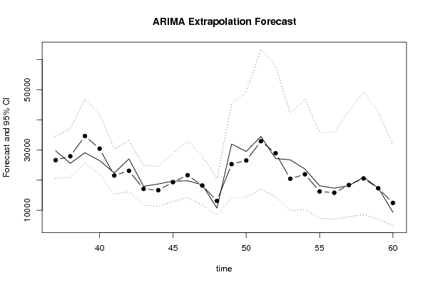
Title produced by software

ARIMA Forecasting

Date of computation

Tue, 28 Dec 2010 17:32:12 +0000

Cite this page as follows

Statistical Computations at FreeStatistics.org, Office for Research Development and Education, URL https://freestatistics.org/blog/index.php?v=date/2010/Dec/28/t1293557462iavn08iueiffx0v.htm/, Retrieved Fri, 03 May 2024 08:08:42 +0000

Statistical Computations at FreeStatistics.org, Office for Research Development and Education, URL https://freestatistics.org/blog/index.php?pk=116441, Retrieved Fri, 03 May 2024 08:08:42 +0000

QR Codes:

Paste this QR Code to cite your computation.

Original text written by user:

IsPrivate?

No (this computation is public)

User-defined keywords

mathias.deruysscher@student.lessius.eu

Estimated Impact

145

Family? (F = Feedback message, R = changed R code, M = changed R Module, P = changed Parameters, D = changed Data)

-     [Multiple Regression] [Q1 The Seatbeltlaw] [2007-11-14 19:27:43] [8cd6641b921d30ebe00b648d1481bba0]
- RM D  [Multiple Regression] [Seatbelt] [2009-11-12 14:06:21] [b98453cac15ba1066b407e146608df68]
- R PD    [Multiple Regression] [] [2009-11-19 08:06:13] [639dd97b6eeebe46a3c92d62cb04fb95]
- RMPD      [ARIMA Forecasting] [] [2009-12-14 08:41:55] [639dd97b6eeebe46a3c92d62cb04fb95]
-   PD        [ARIMA Forecasting] [] [2009-12-19 10:06:44] [ea26ab7ea3bba830cfeb08d06278d52c]
- R PD          [ARIMA Forecasting] [Arima forecast 6 ...] [2009-12-21 17:12:24] [9dbb467a28ad600d808a4e47d5e0774e]
-   P             [ARIMA Forecasting] [Arima forecast 24...] [2009-12-21 17:25:53] [9dbb467a28ad600d808a4e47d5e0774e]
-                     [ARIMA Forecasting] [paper] [2010-12-28 17:32:12] [a4671b53c9c003ef222bf9d29c2203ca] [Current]

Feedback Forum

Post a new message

Dataseries X:

Download CSV

Histogram

Boxplots

Summary of computational transaction
Raw Input	view raw input (R code)
Raw Output	view raw output of R engine
Computing time	2 seconds
R Server	'Sir Ronald Aylmer Fisher' @ 193.190.124.24

\begin{tabular}{lllllllll}
\hline
Summary of computational transaction \tabularnewline
Raw Input & view raw input (R code)  \tabularnewline
Raw Output & view raw output of R engine  \tabularnewline
Computing time & 2 seconds \tabularnewline
R Server & 'Sir Ronald Aylmer Fisher' @ 193.190.124.24 \tabularnewline
\hline
\end{tabular}
%Source: https://freestatistics.org/blog/index.php?pk=116441&T=0

[TABLE]
[ROW][C]Summary of computational transaction[/C][/ROW]
[ROW][C]Raw Input[/C][C]view raw input (R code) [/C][/ROW]
[ROW][C]Raw Output[/C][C]view raw output of R engine [/C][/ROW]
[ROW][C]Computing time[/C][C]2 seconds[/C][/ROW]
[ROW][C]R Server[/C][C]'Sir Ronald Aylmer Fisher' @ 193.190.124.24[/C][/ROW]
[/TABLE]
Source: https://freestatistics.org/blog/index.php?pk=116441&T=0

Globally Unique Identifier (entire table): ba.freestatistics.org/blog/index.php?pk=116441&T=0

As an alternative you can also use a QR Code:

The GUIDs for individual cells are displayed in the table below:

Summary of computational transaction
Raw Input	view raw input (R code)
Raw Output	view raw output of R engine
Computing time	2 seconds
R Server	'Sir Ronald Aylmer Fisher' @ 193.190.124.24

Univariate ARIMA Extrapolation Forecast
time	Y[t]	F[t]	95% LB	95% UB	p-value(H0: Y[t] = F[t])	P(F[t]>Y[t-1])	P(F[t]>Y[t-s])	P(F[t]>Y[36])
24	15548	-	-	-	-	-	-	-
25	28029	-	-	-	-	-	-	-
26	29383	-	-	-	-	-	-	-
27	36438	-	-	-	-	-	-	-
28	32034	-	-	-	-	-	-	-
29	22679	-	-	-	-	-	-	-
30	24319	-	-	-	-	-	-	-
31	18004	-	-	-	-	-	-	-
32	17537	-	-	-	-	-	-	-
33	20366	-	-	-	-	-	-	-
34	22782	-	-	-	-	-	-	-
35	19169	-	-	-	-	-	-	-
36	13807	-	-	-	-	-	-	-
37	29743	26633.4321	20516.9751	34573.3083	0.2214	0.9992	0.3652	0.9992
38	25591	27920.0163	21042.5065	37045.3637	0.3085	0.3477	0.3767	0.9988
39	29096	34623.7468	25570.3057	46882.6559	0.1884	0.9257	0.3859	0.9996
40	26482	30439.0226	22056.0405	42008.179	0.2513	0.59	0.3935	0.9976
41	22405	21549.8094	15336.8801	30279.5797	0.4239	0.1341	0.3999	0.9589
42	27044	23108.1535	16167.6771	33028.0445	0.2184	0.5552	0.4055	0.967
43	17970	17107.5783	11776.0058	24853.0138	0.4136	0.006	0.4103	0.7982
44	18730	16663.8303	11292.9449	24589.09	0.3047	0.3733	0.4145	0.7601
45	19684	19351.974	12919.3922	28987.3463	0.4731	0.5503	0.4183	0.8703
46	19785	21647.681	14244.4615	32898.5475	0.3728	0.6339	0.4217	0.914
47	18479	18214.5728	11819.0202	28070.9107	0.479	0.3774	0.4247	0.8096
48	10698	13119.5475	8398.4552	20494.5459	0.2599	0.0772	0.4275	0.4275
49	31956	25307.3497	14176.1018	45178.9894	0.256	0.9252	0.3309	0.8717
50	29506	26529.8747	14282.434	49279.7131	0.3988	0.3201	0.5322	0.8635
51	34506	32899.8255	17063.1162	63434.985	0.4589	0.5862	0.5964	0.8898
52	27165	28923.4593	14480.5527	57771.7245	0.4525	0.3522	0.5659	0.8478
53	26736	20476.8413	9913.1816	42297.3214	0.287	0.274	0.4312	0.7255
54	23691	21957.5953	10294.2809	46835.325	0.4457	0.3533	0.3443	0.7396
55	18157	16255.7895	7390.0518	35757.624	0.4242	0.2275	0.4316	0.5972
56	17328	15834.1358	6988.194	35877.6327	0.4419	0.4102	0.3885	0.5786
57	18205	18388.4364	7886.7257	42873.8882	0.4941	0.5338	0.4587	0.6431
58	20995	20569.8399	8581.6379	49305.0766	0.4884	0.5641	0.5213	0.6777
59	17382	17307.6666	7029.6506	42613.1171	0.4977	0.3876	0.4639	0.6069
60	9367	12466.3234	4933.171	31502.9052	0.3748	0.3064	0.5722	0.4451

\begin{tabular}{lllllllll}
\hline
Univariate ARIMA Extrapolation Forecast \tabularnewline
time & Y[t] & F[t] & 95% LB & 95% UB & p-value(H0: Y[t] = F[t]) & P(F[t]>Y[t-1]) & P(F[t]>Y[t-s]) & P(F[t]>Y[36]) \tabularnewline
24 & 15548 & - & - & - & - & - & - & - \tabularnewline
25 & 28029 & - & - & - & - & - & - & - \tabularnewline
26 & 29383 & - & - & - & - & - & - & - \tabularnewline
27 & 36438 & - & - & - & - & - & - & - \tabularnewline
28 & 32034 & - & - & - & - & - & - & - \tabularnewline
29 & 22679 & - & - & - & - & - & - & - \tabularnewline
30 & 24319 & - & - & - & - & - & - & - \tabularnewline
31 & 18004 & - & - & - & - & - & - & - \tabularnewline
32 & 17537 & - & - & - & - & - & - & - \tabularnewline
33 & 20366 & - & - & - & - & - & - & - \tabularnewline
34 & 22782 & - & - & - & - & - & - & - \tabularnewline
35 & 19169 & - & - & - & - & - & - & - \tabularnewline
36 & 13807 & - & - & - & - & - & - & - \tabularnewline
37 & 29743 & 26633.4321 & 20516.9751 & 34573.3083 & 0.2214 & 0.9992 & 0.3652 & 0.9992 \tabularnewline
38 & 25591 & 27920.0163 & 21042.5065 & 37045.3637 & 0.3085 & 0.3477 & 0.3767 & 0.9988 \tabularnewline
39 & 29096 & 34623.7468 & 25570.3057 & 46882.6559 & 0.1884 & 0.9257 & 0.3859 & 0.9996 \tabularnewline
40 & 26482 & 30439.0226 & 22056.0405 & 42008.179 & 0.2513 & 0.59 & 0.3935 & 0.9976 \tabularnewline
41 & 22405 & 21549.8094 & 15336.8801 & 30279.5797 & 0.4239 & 0.1341 & 0.3999 & 0.9589 \tabularnewline
42 & 27044 & 23108.1535 & 16167.6771 & 33028.0445 & 0.2184 & 0.5552 & 0.4055 & 0.967 \tabularnewline
43 & 17970 & 17107.5783 & 11776.0058 & 24853.0138 & 0.4136 & 0.006 & 0.4103 & 0.7982 \tabularnewline
44 & 18730 & 16663.8303 & 11292.9449 & 24589.09 & 0.3047 & 0.3733 & 0.4145 & 0.7601 \tabularnewline
45 & 19684 & 19351.974 & 12919.3922 & 28987.3463 & 0.4731 & 0.5503 & 0.4183 & 0.8703 \tabularnewline
46 & 19785 & 21647.681 & 14244.4615 & 32898.5475 & 0.3728 & 0.6339 & 0.4217 & 0.914 \tabularnewline
47 & 18479 & 18214.5728 & 11819.0202 & 28070.9107 & 0.479 & 0.3774 & 0.4247 & 0.8096 \tabularnewline
48 & 10698 & 13119.5475 & 8398.4552 & 20494.5459 & 0.2599 & 0.0772 & 0.4275 & 0.4275 \tabularnewline
49 & 31956 & 25307.3497 & 14176.1018 & 45178.9894 & 0.256 & 0.9252 & 0.3309 & 0.8717 \tabularnewline
50 & 29506 & 26529.8747 & 14282.434 & 49279.7131 & 0.3988 & 0.3201 & 0.5322 & 0.8635 \tabularnewline
51 & 34506 & 32899.8255 & 17063.1162 & 63434.985 & 0.4589 & 0.5862 & 0.5964 & 0.8898 \tabularnewline
52 & 27165 & 28923.4593 & 14480.5527 & 57771.7245 & 0.4525 & 0.3522 & 0.5659 & 0.8478 \tabularnewline
53 & 26736 & 20476.8413 & 9913.1816 & 42297.3214 & 0.287 & 0.274 & 0.4312 & 0.7255 \tabularnewline
54 & 23691 & 21957.5953 & 10294.2809 & 46835.325 & 0.4457 & 0.3533 & 0.3443 & 0.7396 \tabularnewline
55 & 18157 & 16255.7895 & 7390.0518 & 35757.624 & 0.4242 & 0.2275 & 0.4316 & 0.5972 \tabularnewline
56 & 17328 & 15834.1358 & 6988.194 & 35877.6327 & 0.4419 & 0.4102 & 0.3885 & 0.5786 \tabularnewline
57 & 18205 & 18388.4364 & 7886.7257 & 42873.8882 & 0.4941 & 0.5338 & 0.4587 & 0.6431 \tabularnewline
58 & 20995 & 20569.8399 & 8581.6379 & 49305.0766 & 0.4884 & 0.5641 & 0.5213 & 0.6777 \tabularnewline
59 & 17382 & 17307.6666 & 7029.6506 & 42613.1171 & 0.4977 & 0.3876 & 0.4639 & 0.6069 \tabularnewline
60 & 9367 & 12466.3234 & 4933.171 & 31502.9052 & 0.3748 & 0.3064 & 0.5722 & 0.4451 \tabularnewline
\hline
\end{tabular}
%Source: https://freestatistics.org/blog/index.php?pk=116441&T=1

[TABLE]
[ROW][C]Univariate ARIMA Extrapolation Forecast[/C][/ROW]
[ROW][C]time[/C][C]Y[t][/C][C]F[t][/C][C]95% LB[/C][C]95% UB[/C][C]p-value(H0: Y[t] = F[t])[/C][C]P(F[t]>Y[t-1])[/C][C]P(F[t]>Y[t-s])[/C][C]P(F[t]>Y[36])[/C][/ROW]
[ROW][C]24[/C][C]15548[/C][C]-[/C][C]-[/C][C]-[/C][C]-[/C][C]-[/C][C]-[/C][C]-[/C][/ROW]
[ROW][C]25[/C][C]28029[/C][C]-[/C][C]-[/C][C]-[/C][C]-[/C][C]-[/C][C]-[/C][C]-[/C][/ROW]
[ROW][C]26[/C][C]29383[/C][C]-[/C][C]-[/C][C]-[/C][C]-[/C][C]-[/C][C]-[/C][C]-[/C][/ROW]
[ROW][C]27[/C][C]36438[/C][C]-[/C][C]-[/C][C]-[/C][C]-[/C][C]-[/C][C]-[/C][C]-[/C][/ROW]
[ROW][C]28[/C][C]32034[/C][C]-[/C][C]-[/C][C]-[/C][C]-[/C][C]-[/C][C]-[/C][C]-[/C][/ROW]
[ROW][C]29[/C][C]22679[/C][C]-[/C][C]-[/C][C]-[/C][C]-[/C][C]-[/C][C]-[/C][C]-[/C][/ROW]
[ROW][C]30[/C][C]24319[/C][C]-[/C][C]-[/C][C]-[/C][C]-[/C][C]-[/C][C]-[/C][C]-[/C][/ROW]
[ROW][C]31[/C][C]18004[/C][C]-[/C][C]-[/C][C]-[/C][C]-[/C][C]-[/C][C]-[/C][C]-[/C][/ROW]
[ROW][C]32[/C][C]17537[/C][C]-[/C][C]-[/C][C]-[/C][C]-[/C][C]-[/C][C]-[/C][C]-[/C][/ROW]
[ROW][C]33[/C][C]20366[/C][C]-[/C][C]-[/C][C]-[/C][C]-[/C][C]-[/C][C]-[/C][C]-[/C][/ROW]
[ROW][C]34[/C][C]22782[/C][C]-[/C][C]-[/C][C]-[/C][C]-[/C][C]-[/C][C]-[/C][C]-[/C][/ROW]
[ROW][C]35[/C][C]19169[/C][C]-[/C][C]-[/C][C]-[/C][C]-[/C][C]-[/C][C]-[/C][C]-[/C][/ROW]
[ROW][C]36[/C][C]13807[/C][C]-[/C][C]-[/C][C]-[/C][C]-[/C][C]-[/C][C]-[/C][C]-[/C][/ROW]
[ROW][C]37[/C][C]29743[/C][C]26633.4321[/C][C]20516.9751[/C][C]34573.3083[/C][C]0.2214[/C][C]0.9992[/C][C]0.3652[/C][C]0.9992[/C][/ROW]
[ROW][C]38[/C][C]25591[/C][C]27920.0163[/C][C]21042.5065[/C][C]37045.3637[/C][C]0.3085[/C][C]0.3477[/C][C]0.3767[/C][C]0.9988[/C][/ROW]
[ROW][C]39[/C][C]29096[/C][C]34623.7468[/C][C]25570.3057[/C][C]46882.6559[/C][C]0.1884[/C][C]0.9257[/C][C]0.3859[/C][C]0.9996[/C][/ROW]
[ROW][C]40[/C][C]26482[/C][C]30439.0226[/C][C]22056.0405[/C][C]42008.179[/C][C]0.2513[/C][C]0.59[/C][C]0.3935[/C][C]0.9976[/C][/ROW]
[ROW][C]41[/C][C]22405[/C][C]21549.8094[/C][C]15336.8801[/C][C]30279.5797[/C][C]0.4239[/C][C]0.1341[/C][C]0.3999[/C][C]0.9589[/C][/ROW]
[ROW][C]42[/C][C]27044[/C][C]23108.1535[/C][C]16167.6771[/C][C]33028.0445[/C][C]0.2184[/C][C]0.5552[/C][C]0.4055[/C][C]0.967[/C][/ROW]
[ROW][C]43[/C][C]17970[/C][C]17107.5783[/C][C]11776.0058[/C][C]24853.0138[/C][C]0.4136[/C][C]0.006[/C][C]0.4103[/C][C]0.7982[/C][/ROW]
[ROW][C]44[/C][C]18730[/C][C]16663.8303[/C][C]11292.9449[/C][C]24589.09[/C][C]0.3047[/C][C]0.3733[/C][C]0.4145[/C][C]0.7601[/C][/ROW]
[ROW][C]45[/C][C]19684[/C][C]19351.974[/C][C]12919.3922[/C][C]28987.3463[/C][C]0.4731[/C][C]0.5503[/C][C]0.4183[/C][C]0.8703[/C][/ROW]
[ROW][C]46[/C][C]19785[/C][C]21647.681[/C][C]14244.4615[/C][C]32898.5475[/C][C]0.3728[/C][C]0.6339[/C][C]0.4217[/C][C]0.914[/C][/ROW]
[ROW][C]47[/C][C]18479[/C][C]18214.5728[/C][C]11819.0202[/C][C]28070.9107[/C][C]0.479[/C][C]0.3774[/C][C]0.4247[/C][C]0.8096[/C][/ROW]
[ROW][C]48[/C][C]10698[/C][C]13119.5475[/C][C]8398.4552[/C][C]20494.5459[/C][C]0.2599[/C][C]0.0772[/C][C]0.4275[/C][C]0.4275[/C][/ROW]
[ROW][C]49[/C][C]31956[/C][C]25307.3497[/C][C]14176.1018[/C][C]45178.9894[/C][C]0.256[/C][C]0.9252[/C][C]0.3309[/C][C]0.8717[/C][/ROW]
[ROW][C]50[/C][C]29506[/C][C]26529.8747[/C][C]14282.434[/C][C]49279.7131[/C][C]0.3988[/C][C]0.3201[/C][C]0.5322[/C][C]0.8635[/C][/ROW]
[ROW][C]51[/C][C]34506[/C][C]32899.8255[/C][C]17063.1162[/C][C]63434.985[/C][C]0.4589[/C][C]0.5862[/C][C]0.5964[/C][C]0.8898[/C][/ROW]
[ROW][C]52[/C][C]27165[/C][C]28923.4593[/C][C]14480.5527[/C][C]57771.7245[/C][C]0.4525[/C][C]0.3522[/C][C]0.5659[/C][C]0.8478[/C][/ROW]
[ROW][C]53[/C][C]26736[/C][C]20476.8413[/C][C]9913.1816[/C][C]42297.3214[/C][C]0.287[/C][C]0.274[/C][C]0.4312[/C][C]0.7255[/C][/ROW]
[ROW][C]54[/C][C]23691[/C][C]21957.5953[/C][C]10294.2809[/C][C]46835.325[/C][C]0.4457[/C][C]0.3533[/C][C]0.3443[/C][C]0.7396[/C][/ROW]
[ROW][C]55[/C][C]18157[/C][C]16255.7895[/C][C]7390.0518[/C][C]35757.624[/C][C]0.4242[/C][C]0.2275[/C][C]0.4316[/C][C]0.5972[/C][/ROW]
[ROW][C]56[/C][C]17328[/C][C]15834.1358[/C][C]6988.194[/C][C]35877.6327[/C][C]0.4419[/C][C]0.4102[/C][C]0.3885[/C][C]0.5786[/C][/ROW]
[ROW][C]57[/C][C]18205[/C][C]18388.4364[/C][C]7886.7257[/C][C]42873.8882[/C][C]0.4941[/C][C]0.5338[/C][C]0.4587[/C][C]0.6431[/C][/ROW]
[ROW][C]58[/C][C]20995[/C][C]20569.8399[/C][C]8581.6379[/C][C]49305.0766[/C][C]0.4884[/C][C]0.5641[/C][C]0.5213[/C][C]0.6777[/C][/ROW]
[ROW][C]59[/C][C]17382[/C][C]17307.6666[/C][C]7029.6506[/C][C]42613.1171[/C][C]0.4977[/C][C]0.3876[/C][C]0.4639[/C][C]0.6069[/C][/ROW]
[ROW][C]60[/C][C]9367[/C][C]12466.3234[/C][C]4933.171[/C][C]31502.9052[/C][C]0.3748[/C][C]0.3064[/C][C]0.5722[/C][C]0.4451[/C][/ROW]
[/TABLE]
Source: https://freestatistics.org/blog/index.php?pk=116441&T=1

Globally Unique Identifier (entire table): ba.freestatistics.org/blog/index.php?pk=116441&T=1

As an alternative you can also use a QR Code:

The GUIDs for individual cells are displayed in the table below:

Univariate ARIMA Extrapolation Forecast
time	Y[t]	F[t]	95% LB	95% UB	p-value(H0: Y[t] = F[t])	P(F[t]>Y[t-1])	P(F[t]>Y[t-s])	P(F[t]>Y[36])
24	15548	-	-	-	-	-	-	-
25	28029	-	-	-	-	-	-	-
26	29383	-	-	-	-	-	-	-
27	36438	-	-	-	-	-	-	-
28	32034	-	-	-	-	-	-	-
29	22679	-	-	-	-	-	-	-
30	24319	-	-	-	-	-	-	-
31	18004	-	-	-	-	-	-	-
32	17537	-	-	-	-	-	-	-
33	20366	-	-	-	-	-	-	-
34	22782	-	-	-	-	-	-	-
35	19169	-	-	-	-	-	-	-
36	13807	-	-	-	-	-	-	-
37	29743	26633.4321	20516.9751	34573.3083	0.2214	0.9992	0.3652	0.9992
38	25591	27920.0163	21042.5065	37045.3637	0.3085	0.3477	0.3767	0.9988
39	29096	34623.7468	25570.3057	46882.6559	0.1884	0.9257	0.3859	0.9996
40	26482	30439.0226	22056.0405	42008.179	0.2513	0.59	0.3935	0.9976
41	22405	21549.8094	15336.8801	30279.5797	0.4239	0.1341	0.3999	0.9589
42	27044	23108.1535	16167.6771	33028.0445	0.2184	0.5552	0.4055	0.967
43	17970	17107.5783	11776.0058	24853.0138	0.4136	0.006	0.4103	0.7982
44	18730	16663.8303	11292.9449	24589.09	0.3047	0.3733	0.4145	0.7601
45	19684	19351.974	12919.3922	28987.3463	0.4731	0.5503	0.4183	0.8703
46	19785	21647.681	14244.4615	32898.5475	0.3728	0.6339	0.4217	0.914
47	18479	18214.5728	11819.0202	28070.9107	0.479	0.3774	0.4247	0.8096
48	10698	13119.5475	8398.4552	20494.5459	0.2599	0.0772	0.4275	0.4275
49	31956	25307.3497	14176.1018	45178.9894	0.256	0.9252	0.3309	0.8717
50	29506	26529.8747	14282.434	49279.7131	0.3988	0.3201	0.5322	0.8635
51	34506	32899.8255	17063.1162	63434.985	0.4589	0.5862	0.5964	0.8898
52	27165	28923.4593	14480.5527	57771.7245	0.4525	0.3522	0.5659	0.8478
53	26736	20476.8413	9913.1816	42297.3214	0.287	0.274	0.4312	0.7255
54	23691	21957.5953	10294.2809	46835.325	0.4457	0.3533	0.3443	0.7396
55	18157	16255.7895	7390.0518	35757.624	0.4242	0.2275	0.4316	0.5972
56	17328	15834.1358	6988.194	35877.6327	0.4419	0.4102	0.3885	0.5786
57	18205	18388.4364	7886.7257	42873.8882	0.4941	0.5338	0.4587	0.6431
58	20995	20569.8399	8581.6379	49305.0766	0.4884	0.5641	0.5213	0.6777
59	17382	17307.6666	7029.6506	42613.1171	0.4977	0.3876	0.4639	0.6069
60	9367	12466.3234	4933.171	31502.9052	0.3748	0.3064	0.5722	0.4451

Univariate ARIMA Extrapolation Forecast Performance
time	% S.E.	PE	MAPE	Sq.E	MSE	RMSE
37	0.1521	0.1168	0	9669412.4685	0	0
38	0.1668	-0.0834	0.1001	5424316.7241	7546864.5963	2747.1557
39	0.1806	-0.1597	0.1199	30555984.7369	15216571.3098	3900.8424
40	0.1939	-0.13	0.1225	15658027.7794	15326935.4272	3914.963
41	0.2067	0.0397	0.1059	731351.0155	12407818.5449	3522.4734
42	0.219	0.1703	0.1166	15490887.3884	12921663.3521	3594.6715
43	0.231	0.0504	0.1072	743771.2181	11181964.4759	3343.9444
44	0.2427	0.124	0.1093	4269057.3151	10317851.0808	3212.1412
45	0.254	0.0172	0.099	110241.2863	9183672.2147	3030.4574
46	0.2652	-0.086	0.0977	3469580.4492	8612263.0382	2934.6657
47	0.2761	0.0145	0.0902	69921.7613	7835686.5584	2799.2296
48	0.2868	-0.1846	0.098	5863892.3383	7671370.3734	2769.7239
49	0.4006	0.2627	0.1107	44204550.2588	10481614.98	3237.5322
50	0.4375	0.1122	0.1108	8857321.9095	10365594.0464	3219.5643
51	0.4735	0.0488	0.1067	2579796.4162	9846540.8711	3137.9198
52	0.5089	-0.0608	0.1038	3092179.2229	9424393.268	3069.9175
53	0.5437	0.3057	0.1157	39177067.6356	11174550.5838	3342.8357
54	0.5781	0.0789	0.1136	3004691.8909	10720669.5453	3274.2434
55	0.6121	0.117	0.1138	3614601.2497	10346665.9508	3216.6234
56	0.6458	0.0943	0.1128	2231630.2395	9940914.1652	3152.9215
57	0.6794	-0.01	0.1079	33648.9257	9469139.63	3077.1967
58	0.7127	0.0207	0.104	180761.1332	9046940.6074	3007.8133
59	0.746	0.0043	0.0996	5525.454	8653835.6008	2941.7402
60	0.7791	-0.2486	0.1059	9605805.3837	8693501.0084	2948.4744

\begin{tabular}{lllllllll}
\hline
Univariate ARIMA Extrapolation Forecast Performance \tabularnewline
time & % S.E. & PE & MAPE & Sq.E & MSE & RMSE \tabularnewline
37 & 0.1521 & 0.1168 & 0 & 9669412.4685 & 0 & 0 \tabularnewline
38 & 0.1668 & -0.0834 & 0.1001 & 5424316.7241 & 7546864.5963 & 2747.1557 \tabularnewline
39 & 0.1806 & -0.1597 & 0.1199 & 30555984.7369 & 15216571.3098 & 3900.8424 \tabularnewline
40 & 0.1939 & -0.13 & 0.1225 & 15658027.7794 & 15326935.4272 & 3914.963 \tabularnewline
41 & 0.2067 & 0.0397 & 0.1059 & 731351.0155 & 12407818.5449 & 3522.4734 \tabularnewline
42 & 0.219 & 0.1703 & 0.1166 & 15490887.3884 & 12921663.3521 & 3594.6715 \tabularnewline
43 & 0.231 & 0.0504 & 0.1072 & 743771.2181 & 11181964.4759 & 3343.9444 \tabularnewline
44 & 0.2427 & 0.124 & 0.1093 & 4269057.3151 & 10317851.0808 & 3212.1412 \tabularnewline
45 & 0.254 & 0.0172 & 0.099 & 110241.2863 & 9183672.2147 & 3030.4574 \tabularnewline
46 & 0.2652 & -0.086 & 0.0977 & 3469580.4492 & 8612263.0382 & 2934.6657 \tabularnewline
47 & 0.2761 & 0.0145 & 0.0902 & 69921.7613 & 7835686.5584 & 2799.2296 \tabularnewline
48 & 0.2868 & -0.1846 & 0.098 & 5863892.3383 & 7671370.3734 & 2769.7239 \tabularnewline
49 & 0.4006 & 0.2627 & 0.1107 & 44204550.2588 & 10481614.98 & 3237.5322 \tabularnewline
50 & 0.4375 & 0.1122 & 0.1108 & 8857321.9095 & 10365594.0464 & 3219.5643 \tabularnewline
51 & 0.4735 & 0.0488 & 0.1067 & 2579796.4162 & 9846540.8711 & 3137.9198 \tabularnewline
52 & 0.5089 & -0.0608 & 0.1038 & 3092179.2229 & 9424393.268 & 3069.9175 \tabularnewline
53 & 0.5437 & 0.3057 & 0.1157 & 39177067.6356 & 11174550.5838 & 3342.8357 \tabularnewline
54 & 0.5781 & 0.0789 & 0.1136 & 3004691.8909 & 10720669.5453 & 3274.2434 \tabularnewline
55 & 0.6121 & 0.117 & 0.1138 & 3614601.2497 & 10346665.9508 & 3216.6234 \tabularnewline
56 & 0.6458 & 0.0943 & 0.1128 & 2231630.2395 & 9940914.1652 & 3152.9215 \tabularnewline
57 & 0.6794 & -0.01 & 0.1079 & 33648.9257 & 9469139.63 & 3077.1967 \tabularnewline
58 & 0.7127 & 0.0207 & 0.104 & 180761.1332 & 9046940.6074 & 3007.8133 \tabularnewline
59 & 0.746 & 0.0043 & 0.0996 & 5525.454 & 8653835.6008 & 2941.7402 \tabularnewline
60 & 0.7791 & -0.2486 & 0.1059 & 9605805.3837 & 8693501.0084 & 2948.4744 \tabularnewline
\hline
\end{tabular}
%Source: https://freestatistics.org/blog/index.php?pk=116441&T=2

[TABLE]
[ROW][C]Univariate ARIMA Extrapolation Forecast Performance[/C][/ROW]
[ROW][C]time[/C][C]% S.E.[/C][C]PE[/C][C]MAPE[/C][C]Sq.E[/C][C]MSE[/C][C]RMSE[/C][/ROW]
[ROW][C]37[/C][C]0.1521[/C][C]0.1168[/C][C]0[/C][C]9669412.4685[/C][C]0[/C][C]0[/C][/ROW]
[ROW][C]38[/C][C]0.1668[/C][C]-0.0834[/C][C]0.1001[/C][C]5424316.7241[/C][C]7546864.5963[/C][C]2747.1557[/C][/ROW]
[ROW][C]39[/C][C]0.1806[/C][C]-0.1597[/C][C]0.1199[/C][C]30555984.7369[/C][C]15216571.3098[/C][C]3900.8424[/C][/ROW]
[ROW][C]40[/C][C]0.1939[/C][C]-0.13[/C][C]0.1225[/C][C]15658027.7794[/C][C]15326935.4272[/C][C]3914.963[/C][/ROW]
[ROW][C]41[/C][C]0.2067[/C][C]0.0397[/C][C]0.1059[/C][C]731351.0155[/C][C]12407818.5449[/C][C]3522.4734[/C][/ROW]
[ROW][C]42[/C][C]0.219[/C][C]0.1703[/C][C]0.1166[/C][C]15490887.3884[/C][C]12921663.3521[/C][C]3594.6715[/C][/ROW]
[ROW][C]43[/C][C]0.231[/C][C]0.0504[/C][C]0.1072[/C][C]743771.2181[/C][C]11181964.4759[/C][C]3343.9444[/C][/ROW]
[ROW][C]44[/C][C]0.2427[/C][C]0.124[/C][C]0.1093[/C][C]4269057.3151[/C][C]10317851.0808[/C][C]3212.1412[/C][/ROW]
[ROW][C]45[/C][C]0.254[/C][C]0.0172[/C][C]0.099[/C][C]110241.2863[/C][C]9183672.2147[/C][C]3030.4574[/C][/ROW]
[ROW][C]46[/C][C]0.2652[/C][C]-0.086[/C][C]0.0977[/C][C]3469580.4492[/C][C]8612263.0382[/C][C]2934.6657[/C][/ROW]
[ROW][C]47[/C][C]0.2761[/C][C]0.0145[/C][C]0.0902[/C][C]69921.7613[/C][C]7835686.5584[/C][C]2799.2296[/C][/ROW]
[ROW][C]48[/C][C]0.2868[/C][C]-0.1846[/C][C]0.098[/C][C]5863892.3383[/C][C]7671370.3734[/C][C]2769.7239[/C][/ROW]
[ROW][C]49[/C][C]0.4006[/C][C]0.2627[/C][C]0.1107[/C][C]44204550.2588[/C][C]10481614.98[/C][C]3237.5322[/C][/ROW]
[ROW][C]50[/C][C]0.4375[/C][C]0.1122[/C][C]0.1108[/C][C]8857321.9095[/C][C]10365594.0464[/C][C]3219.5643[/C][/ROW]
[ROW][C]51[/C][C]0.4735[/C][C]0.0488[/C][C]0.1067[/C][C]2579796.4162[/C][C]9846540.8711[/C][C]3137.9198[/C][/ROW]
[ROW][C]52[/C][C]0.5089[/C][C]-0.0608[/C][C]0.1038[/C][C]3092179.2229[/C][C]9424393.268[/C][C]3069.9175[/C][/ROW]
[ROW][C]53[/C][C]0.5437[/C][C]0.3057[/C][C]0.1157[/C][C]39177067.6356[/C][C]11174550.5838[/C][C]3342.8357[/C][/ROW]
[ROW][C]54[/C][C]0.5781[/C][C]0.0789[/C][C]0.1136[/C][C]3004691.8909[/C][C]10720669.5453[/C][C]3274.2434[/C][/ROW]
[ROW][C]55[/C][C]0.6121[/C][C]0.117[/C][C]0.1138[/C][C]3614601.2497[/C][C]10346665.9508[/C][C]3216.6234[/C][/ROW]
[ROW][C]56[/C][C]0.6458[/C][C]0.0943[/C][C]0.1128[/C][C]2231630.2395[/C][C]9940914.1652[/C][C]3152.9215[/C][/ROW]
[ROW][C]57[/C][C]0.6794[/C][C]-0.01[/C][C]0.1079[/C][C]33648.9257[/C][C]9469139.63[/C][C]3077.1967[/C][/ROW]
[ROW][C]58[/C][C]0.7127[/C][C]0.0207[/C][C]0.104[/C][C]180761.1332[/C][C]9046940.6074[/C][C]3007.8133[/C][/ROW]
[ROW][C]59[/C][C]0.746[/C][C]0.0043[/C][C]0.0996[/C][C]5525.454[/C][C]8653835.6008[/C][C]2941.7402[/C][/ROW]
[ROW][C]60[/C][C]0.7791[/C][C]-0.2486[/C][C]0.1059[/C][C]9605805.3837[/C][C]8693501.0084[/C][C]2948.4744[/C][/ROW]
[/TABLE]
Source: https://freestatistics.org/blog/index.php?pk=116441&T=2

Globally Unique Identifier (entire table): ba.freestatistics.org/blog/index.php?pk=116441&T=2

As an alternative you can also use a QR Code:

The GUIDs for individual cells are displayed in the table below:

Univariate ARIMA Extrapolation Forecast Performance
time	% S.E.	PE	MAPE	Sq.E	MSE	RMSE
37	0.1521	0.1168	0	9669412.4685	0	0
38	0.1668	-0.0834	0.1001	5424316.7241	7546864.5963	2747.1557
39	0.1806	-0.1597	0.1199	30555984.7369	15216571.3098	3900.8424
40	0.1939	-0.13	0.1225	15658027.7794	15326935.4272	3914.963
41	0.2067	0.0397	0.1059	731351.0155	12407818.5449	3522.4734
42	0.219	0.1703	0.1166	15490887.3884	12921663.3521	3594.6715
43	0.231	0.0504	0.1072	743771.2181	11181964.4759	3343.9444
44	0.2427	0.124	0.1093	4269057.3151	10317851.0808	3212.1412
45	0.254	0.0172	0.099	110241.2863	9183672.2147	3030.4574
46	0.2652	-0.086	0.0977	3469580.4492	8612263.0382	2934.6657
47	0.2761	0.0145	0.0902	69921.7613	7835686.5584	2799.2296
48	0.2868	-0.1846	0.098	5863892.3383	7671370.3734	2769.7239
49	0.4006	0.2627	0.1107	44204550.2588	10481614.98	3237.5322
50	0.4375	0.1122	0.1108	8857321.9095	10365594.0464	3219.5643
51	0.4735	0.0488	0.1067	2579796.4162	9846540.8711	3137.9198
52	0.5089	-0.0608	0.1038	3092179.2229	9424393.268	3069.9175
53	0.5437	0.3057	0.1157	39177067.6356	11174550.5838	3342.8357
54	0.5781	0.0789	0.1136	3004691.8909	10720669.5453	3274.2434
55	0.6121	0.117	0.1138	3614601.2497	10346665.9508	3216.6234
56	0.6458	0.0943	0.1128	2231630.2395	9940914.1652	3152.9215
57	0.6794	-0.01	0.1079	33648.9257	9469139.63	3077.1967
58	0.7127	0.0207	0.104	180761.1332	9046940.6074	3007.8133
59	0.746	0.0043	0.0996	5525.454	8653835.6008	2941.7402
60	0.7791	-0.2486	0.1059	9605805.3837	8693501.0084	2948.4744

Figure 1

PNG link

Postscript link

PDF link

Figure 2

PNG link

Postscript link

PDF link

Parameters (Session):

par1 = 24 ; par2 = 0.0 ; par3 = 1 ; par4 = 1 ; par5 = 12 ; par6 = 0 ; par7 = 1 ; par8 = 0 ; par9 = 0 ; par10 = FALSE ;

Parameters (R input):

par1 = 24 ; par2 = 0.0 ; par3 = 1 ; par4 = 1 ; par5 = 12 ; par6 = 0 ; par7 = 1 ; par8 = 0 ; par9 = 0 ; par10 = FALSE ;

R code (references can be found in the software module):

par1 <- as.numeric(par1) #cut off periods
par2 <- as.numeric(par2) #lambda
par3 <- as.numeric(par3) #degree of non-seasonal differencing
par4 <- as.numeric(par4) #degree of seasonal differencing
par5 <- as.numeric(par5) #seasonal period
par6 <- as.numeric(par6) #p
par7 <- as.numeric(par7) #q
par8 <- as.numeric(par8) #P
par9 <- as.numeric(par9) #Q
if (par10 == 'TRUE') par10 <- TRUE
if (par10 == 'FALSE') par10 <- FALSE
if (par2 == 0) x <- log(x)
if (par2 != 0) x <- x^par2
lx <- length(x)
first <- lx - 2*par1
nx <- lx - par1
nx1 <- nx + 1
fx <- lx - nx
if (fx < 1) {
fx <- par5
nx1 <- lx + fx - 1
first <- lx - 2*fx
}
first <- 1
if (fx < 3) fx <- round(lx/10,0)
(arima.out <- arima(x[1:nx], order=c(par6,par3,par7), seasonal=list(order=c(par8,par4,par9), period=par5), include.mean=par10, method='ML'))
(forecast <- predict(arima.out,par1))
(lb <- forecast$pred - 1.96 * forecast$se)
(ub <- forecast$pred + 1.96 * forecast$se)
if (par2 == 0) {
x <- exp(x)
forecast$pred <- exp(forecast$pred)
lb <- exp(lb)
ub <- exp(ub)
}
if (par2 != 0) {
x <- x^(1/par2)
forecast$pred <- forecast$pred^(1/par2)
lb <- lb^(1/par2)
ub <- ub^(1/par2)
}
if (par2 < 0) {
olb <- lb
lb <- ub
ub <- olb
}
(actandfor <- c(x[1:nx], forecast$pred))
(perc.se <- (ub-forecast$pred)/1.96/forecast$pred)
bitmap(file='test1.png')
opar <- par(mar=c(4,4,2,2),las=1)
ylim <- c( min(x[first:nx],lb), max(x[first:nx],ub))
plot(x,ylim=ylim,type='n',xlim=c(first,lx))
usr <- par('usr')
rect(usr[1],usr[3],nx+1,usr[4],border=NA,col='lemonchiffon')
rect(nx1,usr[3],usr[2],usr[4],border=NA,col='lavender')
abline(h= (-3:3)*2 , col ='gray', lty =3)
polygon( c(nx1:lx,lx:nx1), c(lb,rev(ub)), col = 'orange', lty=2,border=NA)
lines(nx1:lx, lb , lty=2)
lines(nx1:lx, ub , lty=2)
lines(x, lwd=2)
lines(nx1:lx, forecast$pred , lwd=2 , col ='white')
box()
par(opar)
dev.off()
prob.dec <- array(NA, dim=fx)
prob.sdec <- array(NA, dim=fx)
prob.ldec <- array(NA, dim=fx)
prob.pval <- array(NA, dim=fx)
perf.pe <- array(0, dim=fx)
perf.mape <- array(0, dim=fx)
perf.mape1 <- array(0, dim=fx)
perf.se <- array(0, dim=fx)
perf.mse <- array(0, dim=fx)
perf.mse1 <- array(0, dim=fx)
perf.rmse <- array(0, dim=fx)
for (i in 1:fx) {
locSD <- (ub[i] - forecast$pred[i]) / 1.96
perf.pe[i] = (x[nx+i] - forecast$pred[i]) / forecast$pred[i]
perf.se[i] = (x[nx+i] - forecast$pred[i])^2
prob.dec[i] = pnorm((x[nx+i-1] - forecast$pred[i]) / locSD)
prob.sdec[i] = pnorm((x[nx+i-par5] - forecast$pred[i]) / locSD)
prob.ldec[i] = pnorm((x[nx] - forecast$pred[i]) / locSD)
prob.pval[i] = pnorm(abs(x[nx+i] - forecast$pred[i]) / locSD)
}
perf.mape[1] = abs(perf.pe[1])
perf.mse[1] = abs(perf.se[1])
for (i in 2:fx) {
perf.mape[i] = perf.mape[i-1] + abs(perf.pe[i])
perf.mape1[i] = perf.mape[i] / i
perf.mse[i] = perf.mse[i-1] + perf.se[i]
perf.mse1[i] = perf.mse[i] / i
}
perf.rmse = sqrt(perf.mse1)
bitmap(file='test2.png')
plot(forecast$pred, pch=19, type='b',main='ARIMA Extrapolation Forecast', ylab='Forecast and 95% CI', xlab='time',ylim=c(min(lb),max(ub)))
dum <- forecast$pred
dum[1:par1] <- x[(nx+1):lx]
lines(dum, lty=1)
lines(ub,lty=3)
lines(lb,lty=3)
dev.off()
load(file='createtable')
a<-table.start()
a<-table.row.start(a)
a<-table.element(a,'Univariate ARIMA Extrapolation Forecast',9,TRUE)
a<-table.row.end(a)
a<-table.row.start(a)
a<-table.element(a,'time',1,header=TRUE)
a<-table.element(a,'Y[t]',1,header=TRUE)
a<-table.element(a,'F[t]',1,header=TRUE)
a<-table.element(a,'95% LB',1,header=TRUE)
a<-table.element(a,'95% UB',1,header=TRUE)
a<-table.element(a,'p-value
(H0: Y[t] = F[t])',1,header=TRUE)
a<-table.element(a,'P(F[t]>Y[t-1])',1,header=TRUE)
a<-table.element(a,'P(F[t]>Y[t-s])',1,header=TRUE)
mylab <- paste('P(F[t]>Y[',nx,sep='')
mylab <- paste(mylab,'])',sep='')
a<-table.element(a,mylab,1,header=TRUE)
a<-table.row.end(a)
for (i in (nx-par5):nx) {
a<-table.row.start(a)
a<-table.element(a,i,header=TRUE)
a<-table.element(a,x[i])
a<-table.element(a,'-')
a<-table.element(a,'-')
a<-table.element(a,'-')
a<-table.element(a,'-')
a<-table.element(a,'-')
a<-table.element(a,'-')
a<-table.element(a,'-')
a<-table.row.end(a)
}
for (i in 1:fx) {
a<-table.row.start(a)
a<-table.element(a,nx+i,header=TRUE)
a<-table.element(a,round(x[nx+i],4))
a<-table.element(a,round(forecast$pred[i],4))
a<-table.element(a,round(lb[i],4))
a<-table.element(a,round(ub[i],4))
a<-table.element(a,round((1-prob.pval[i]),4))
a<-table.element(a,round((1-prob.dec[i]),4))
a<-table.element(a,round((1-prob.sdec[i]),4))
a<-table.element(a,round((1-prob.ldec[i]),4))
a<-table.row.end(a)
}
a<-table.end(a)
table.save(a,file='mytable.tab')
a<-table.start()
a<-table.row.start(a)
a<-table.element(a,'Univariate ARIMA Extrapolation Forecast Performance',7,TRUE)
a<-table.row.end(a)
a<-table.row.start(a)
a<-table.element(a,'time',1,header=TRUE)
a<-table.element(a,'% S.E.',1,header=TRUE)
a<-table.element(a,'PE',1,header=TRUE)
a<-table.element(a,'MAPE',1,header=TRUE)
a<-table.element(a,'Sq.E',1,header=TRUE)
a<-table.element(a,'MSE',1,header=TRUE)
a<-table.element(a,'RMSE',1,header=TRUE)
a<-table.row.end(a)
for (i in 1:fx) {
a<-table.row.start(a)
a<-table.element(a,nx+i,header=TRUE)
a<-table.element(a,round(perc.se[i],4))
a<-table.element(a,round(perf.pe[i],4))
a<-table.element(a,round(perf.mape1[i],4))
a<-table.element(a,round(perf.se[i],4))
a<-table.element(a,round(perf.mse1[i],4))
a<-table.element(a,round(perf.rmse[i],4))
a<-table.row.end(a)
}
a<-table.end(a)
table.save(a,file='mytable1.tab')

Free Statistics

Description of Statistical Computation

Tree of Dependent Computations

Dataset

Tables (Output of Computation)

Figures (Output of Computation)

Input Parameters & R Code