Free Statistics
of Irreproducible Research!
Description of Statistical Computation | |||||||||||||||||||||||||||||||||||||||||||||||||||||||||||||||||||||||||||||||||||||||||||||||||||||||||||||||||||||||||||||||||||||||||||||||||||||||||||||||||||||||||||||||||||||||||||||||||||||||||||||||||||||||||||||||||||||||||||||||||||||||||||||||||||||||||||
|---|---|---|---|---|---|---|---|---|---|---|---|---|---|---|---|---|---|---|---|---|---|---|---|---|---|---|---|---|---|---|---|---|---|---|---|---|---|---|---|---|---|---|---|---|---|---|---|---|---|---|---|---|---|---|---|---|---|---|---|---|---|---|---|---|---|---|---|---|---|---|---|---|---|---|---|---|---|---|---|---|---|---|---|---|---|---|---|---|---|---|---|---|---|---|---|---|---|---|---|---|---|---|---|---|---|---|---|---|---|---|---|---|---|---|---|---|---|---|---|---|---|---|---|---|---|---|---|---|---|---|---|---|---|---|---|---|---|---|---|---|---|---|---|---|---|---|---|---|---|---|---|---|---|---|---|---|---|---|---|---|---|---|---|---|---|---|---|---|---|---|---|---|---|---|---|---|---|---|---|---|---|---|---|---|---|---|---|---|---|---|---|---|---|---|---|---|---|---|---|---|---|---|---|---|---|---|---|---|---|---|---|---|---|---|---|---|---|---|---|---|---|---|---|---|---|---|---|---|---|---|---|---|---|---|---|---|---|---|---|---|---|---|---|---|---|---|---|---|---|---|---|---|---|---|---|---|---|---|---|---|---|---|---|---|---|---|---|
| Author's title | |||||||||||||||||||||||||||||||||||||||||||||||||||||||||||||||||||||||||||||||||||||||||||||||||||||||||||||||||||||||||||||||||||||||||||||||||||||||||||||||||||||||||||||||||||||||||||||||||||||||||||||||||||||||||||||||||||||||||||||||||||||||||||||||||||||||||||
| Author | *The author of this computation has been verified* | ||||||||||||||||||||||||||||||||||||||||||||||||||||||||||||||||||||||||||||||||||||||||||||||||||||||||||||||||||||||||||||||||||||||||||||||||||||||||||||||||||||||||||||||||||||||||||||||||||||||||||||||||||||||||||||||||||||||||||||||||||||||||||||||||||||||||||
| R Software Module | Ian.Hollidayrwasp_Two Factor ANOVA -V2.wasp | ||||||||||||||||||||||||||||||||||||||||||||||||||||||||||||||||||||||||||||||||||||||||||||||||||||||||||||||||||||||||||||||||||||||||||||||||||||||||||||||||||||||||||||||||||||||||||||||||||||||||||||||||||||||||||||||||||||||||||||||||||||||||||||||||||||||||||
| Title produced by software | Two-Way ANOVA | ||||||||||||||||||||||||||||||||||||||||||||||||||||||||||||||||||||||||||||||||||||||||||||||||||||||||||||||||||||||||||||||||||||||||||||||||||||||||||||||||||||||||||||||||||||||||||||||||||||||||||||||||||||||||||||||||||||||||||||||||||||||||||||||||||||||||||
| Date of computation | Wed, 26 May 2010 17:02:24 +0000 | ||||||||||||||||||||||||||||||||||||||||||||||||||||||||||||||||||||||||||||||||||||||||||||||||||||||||||||||||||||||||||||||||||||||||||||||||||||||||||||||||||||||||||||||||||||||||||||||||||||||||||||||||||||||||||||||||||||||||||||||||||||||||||||||||||||||||||
| Cite this page as follows | Statistical Computations at FreeStatistics.org, Office for Research Development and Education, URL https://freestatistics.org/blog/index.php?v=date/2010/May/26/t1274894195nc0qduhoo1uxtyk.htm/, Retrieved Mon, 08 Jun 2026 21:42:03 +0000 | ||||||||||||||||||||||||||||||||||||||||||||||||||||||||||||||||||||||||||||||||||||||||||||||||||||||||||||||||||||||||||||||||||||||||||||||||||||||||||||||||||||||||||||||||||||||||||||||||||||||||||||||||||||||||||||||||||||||||||||||||||||||||||||||||||||||||||
| Statistical Computations at FreeStatistics.org, Office for Research Development and Education, URL https://freestatistics.org/blog/index.php?pk=76523, Retrieved Mon, 08 Jun 2026 21:42:03 +0000 | |||||||||||||||||||||||||||||||||||||||||||||||||||||||||||||||||||||||||||||||||||||||||||||||||||||||||||||||||||||||||||||||||||||||||||||||||||||||||||||||||||||||||||||||||||||||||||||||||||||||||||||||||||||||||||||||||||||||||||||||||||||||||||||||||||||||||||
| QR Codes: | |||||||||||||||||||||||||||||||||||||||||||||||||||||||||||||||||||||||||||||||||||||||||||||||||||||||||||||||||||||||||||||||||||||||||||||||||||||||||||||||||||||||||||||||||||||||||||||||||||||||||||||||||||||||||||||||||||||||||||||||||||||||||||||||||||||||||||
|
| |||||||||||||||||||||||||||||||||||||||||||||||||||||||||||||||||||||||||||||||||||||||||||||||||||||||||||||||||||||||||||||||||||||||||||||||||||||||||||||||||||||||||||||||||||||||||||||||||||||||||||||||||||||||||||||||||||||||||||||||||||||||||||||||||||||||||||
| Original text written by user: | |||||||||||||||||||||||||||||||||||||||||||||||||||||||||||||||||||||||||||||||||||||||||||||||||||||||||||||||||||||||||||||||||||||||||||||||||||||||||||||||||||||||||||||||||||||||||||||||||||||||||||||||||||||||||||||||||||||||||||||||||||||||||||||||||||||||||||
| IsPrivate? | No (this computation is public) | ||||||||||||||||||||||||||||||||||||||||||||||||||||||||||||||||||||||||||||||||||||||||||||||||||||||||||||||||||||||||||||||||||||||||||||||||||||||||||||||||||||||||||||||||||||||||||||||||||||||||||||||||||||||||||||||||||||||||||||||||||||||||||||||||||||||||||
| User-defined keywords | |||||||||||||||||||||||||||||||||||||||||||||||||||||||||||||||||||||||||||||||||||||||||||||||||||||||||||||||||||||||||||||||||||||||||||||||||||||||||||||||||||||||||||||||||||||||||||||||||||||||||||||||||||||||||||||||||||||||||||||||||||||||||||||||||||||||||||
| Estimated Impact | 582 | ||||||||||||||||||||||||||||||||||||||||||||||||||||||||||||||||||||||||||||||||||||||||||||||||||||||||||||||||||||||||||||||||||||||||||||||||||||||||||||||||||||||||||||||||||||||||||||||||||||||||||||||||||||||||||||||||||||||||||||||||||||||||||||||||||||||||||
Tree of Dependent Computations | |||||||||||||||||||||||||||||||||||||||||||||||||||||||||||||||||||||||||||||||||||||||||||||||||||||||||||||||||||||||||||||||||||||||||||||||||||||||||||||||||||||||||||||||||||||||||||||||||||||||||||||||||||||||||||||||||||||||||||||||||||||||||||||||||||||||||||
| Family? (F = Feedback message, R = changed R code, M = changed R Module, P = changed Parameters, D = changed Data) | |||||||||||||||||||||||||||||||||||||||||||||||||||||||||||||||||||||||||||||||||||||||||||||||||||||||||||||||||||||||||||||||||||||||||||||||||||||||||||||||||||||||||||||||||||||||||||||||||||||||||||||||||||||||||||||||||||||||||||||||||||||||||||||||||||||||||||
| - [Two-Way ANOVA] [two-way anova wit...] [2010-05-26 17:02:24] [a9208f4f8d3b118336aae915785f2bd9] [Current] - R PD [Two-Way ANOVA] [ANOVA with good l...] [2010-05-28 23:09:47] [98fd0e87c3eb04e0cc2efde01dbafab6] - R [Variability] [ANOVA with better...] [2010-05-29 09:47:12] [98fd0e87c3eb04e0cc2efde01dbafab6] - R [Variability] [ANOVA with better...] [2010-05-29 09:54:40] [98fd0e87c3eb04e0cc2efde01dbafab6] - R D [Variability] [compendium] [2010-05-30 20:52:28] [4edce1892c378475bb20c4acd224a51d] - R D [Variability] [Trimmed 10%] [2010-05-31 11:11:24] [856c65906cd78e3f7881668c6dfea87f] - R D [Variability] [Trimmed date 10%] [2010-05-31 11:11:52] [885328d98a95a442af53d0763bccf325] - RMPD [] [] [1970-01-01 00:00:00] [166b3b50b14ad81e946931c96c6ff94f] - RMP [Two-Way ANOVA] [] [2010-06-01 23:03:14] [3a572644bd86164a067a2945d748afb7] - R [Variability] [blog 1] [2010-06-02 08:40:04] [c519646407a489a26f129bdc22b2e203] - R [Variability] [SectionA] [2010-06-02 08:40:35] [4edce1892c378475bb20c4acd224a51d] - R [Variability] [Test 1] [2010-06-02 08:40:25] [7d07ebb7f3978280240b500f174a2af2] - R D [Variability] [test 2] [2010-06-02 09:11:16] [7d07ebb7f3978280240b500f174a2af2] - RMPD [Simple Linear Regression] [linear regression] [2010-06-02 09:42:39] [7d07ebb7f3978280240b500f174a2af2] - R [Variability] [Question one] [2010-06-02 08:40:45] [6754037f2a7547483397efade45eb176] - R [Variability] [Question 1] [2010-06-02 08:40:59] [153000c0b3bd367036e4d581452d08df] - R D [Variability] [Question 1ii] [2010-06-02 08:52:01] [153000c0b3bd367036e4d581452d08df] - R [Variability] [Examcompendium] [2010-06-02 08:40:07] [175567c9546e50fd2412bc13fece161f] - R [Variability] [Section A 1 - 1] [2010-06-02 08:40:52] [5cb86ecb659a3920b562748ed004e500] - R [Variability] [adler] [2010-06-02 08:41:42] [f894c941edfbe86ae91b01acfc2a02b5] - R [Variability] [exam] [2010-06-02 08:41:23] [5bdc9e4bd4169daeceaf774f5b9d9a20] - R [Variability] [section A Q1] [2010-06-02 08:41:49] [256a42577f5eb7e9c8a1b74c73a90fa8] - R [Variability] [june exam section...] [2010-06-02 08:41:39] [a2ec18f77143ca7c2255feafca790c81] - R [Variability] [] [2010-06-02 08:41:42] [a6e410a5e6b2ff1e0abc686251520516] - R D [Variability] [exam1] [2010-06-02 08:41:53] [86674042f568b97a0cb1393bb670625c] - R [Variability] [Adler Exam Reprod...] [2010-06-02 08:41:55] [814d7f27257f4c09e0e8a930c67f7fe6] - R [Variability] [] [2010-06-02 08:42:17] [74be16979710d4c4e7c6647856088456] - R [Variability] [Reproduced Analys...] [2010-06-02 08:42:28] [e92f8a4a2b7017be7b51e64bfca3a271] - R [Variability] [reproduction of a...] [2010-06-02 08:42:14] [c3b05d290fad0f2bad0901abbf20f20e] - R [Variability] [Adler Study] [2010-06-02 08:41:57] [74be16979710d4c4e7c6647856088456] - R [Variability] [June exam ANOVA] [2010-06-02 08:42:16] [012a64ac316c94a67eaef3285dac2cf7] - R [Variability] [] [2010-06-02 08:42:05] [a0fd591e63c5cd1c7fa328d28b50e124] - R [Variability] [Adler Study] [2010-06-02 08:41:55] [06b133101696c6b5dc677840451c9976] - R D [Variability] [Adler Adjusted] [2010-06-02 09:17:20] [06b133101696c6b5dc677840451c9976] - R [Variability] [Exam QA1] [2010-06-02 08:43:04] [2cb75f3785cab2383fe897d8b1eb3abc] - R D [Variability] [SUMMER EXAM QA ad...] [2010-06-02 09:21:13] [2cb75f3785cab2383fe897d8b1eb3abc] - R [Variability] [AdvancedStats] [2010-06-02 08:43:30] [7ee8584ae92dbbc2a823887b8397aaa8] - R [Variability] [Section A - ANOVA] [2010-06-02 08:43:24] [8431b2cca73e677c29fb8bfdfc230859] - R [Variability] [Section a q1] [2010-06-02 08:44:23] [d85e8cd4dd2ccdf2c3dfa3761837f774] - R [Variability] [] [2010-06-02 08:42:08] [5937f6f6887339314deaa19552a34d35] - R [Variability] [ANOVA] [2010-06-02 08:44:10] [01668bebb17c5d247271c36324d8beb6] - R [Variability] [ANOVA for attract...] [2010-06-02 09:08:14] [01668bebb17c5d247271c36324d8beb6] - R [Variability] [statsexam] [2010-06-02 08:44:40] [66f61a2d5ef80b1eafe31e5651ad0889] - R [Variability] [adler study] [2010-06-02 08:42:09] [74be16979710d4c4e7c6647856088456] - R [Variability] [adler study] [2010-06-02 08:42:09] [74be16979710d4c4e7c6647856088456] - R [Variability] [Adler] [2010-06-02 08:42:19] [f4cf89988ffad44ee0ca561abbab9122] - R [Variability] [] [2010-06-02 08:45:50] [36cf82ea4074b55afa05ece289b9dfca] - R [Variability] [] [2010-06-02 08:46:11] [bab33aa52cf59fc0c168bbba8dd04cc1] - R [Variability] [Nacy Adler (1973)] [2010-06-02 08:40:58] [166b3b50b14ad81e946931c96c6ff94f] [Truncated] | |||||||||||||||||||||||||||||||||||||||||||||||||||||||||||||||||||||||||||||||||||||||||||||||||||||||||||||||||||||||||||||||||||||||||||||||||||||||||||||||||||||||||||||||||||||||||||||||||||||||||||||||||||||||||||||||||||||||||||||||||||||||||||||||||||||||||||
| Feedback Forum | |||||||||||||||||||||||||||||||||||||||||||||||||||||||||||||||||||||||||||||||||||||||||||||||||||||||||||||||||||||||||||||||||||||||||||||||||||||||||||||||||||||||||||||||||||||||||||||||||||||||||||||||||||||||||||||||||||||||||||||||||||||||||||||||||||||||||||
Post a new message | |||||||||||||||||||||||||||||||||||||||||||||||||||||||||||||||||||||||||||||||||||||||||||||||||||||||||||||||||||||||||||||||||||||||||||||||||||||||||||||||||||||||||||||||||||||||||||||||||||||||||||||||||||||||||||||||||||||||||||||||||||||||||||||||||||||||||||
Dataset | |||||||||||||||||||||||||||||||||||||||||||||||||||||||||||||||||||||||||||||||||||||||||||||||||||||||||||||||||||||||||||||||||||||||||||||||||||||||||||||||||||||||||||||||||||||||||||||||||||||||||||||||||||||||||||||||||||||||||||||||||||||||||||||||||||||||||||
| Dataseries X: | |||||||||||||||||||||||||||||||||||||||||||||||||||||||||||||||||||||||||||||||||||||||||||||||||||||||||||||||||||||||||||||||||||||||||||||||||||||||||||||||||||||||||||||||||||||||||||||||||||||||||||||||||||||||||||||||||||||||||||||||||||||||||||||||||||||||||||
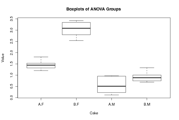
0.28 'A' 'M' 0.95 'A' 'M' 0.96 'A' 'M' 0.97 'A' 'M' 0.40 'A' 'M' 0.18 'A' 'M' 0.12 'A' 'M' 0.62 'A' 'M' 1.81 'A' 'F' 1.51 'A' 'F' 1.41 'A' 'F' 1.39 'A' 'F' 1.20 'A' 'F' 1.55 'A' 'F' 1.48 'A' 'F' 1.25 'A' 'F' 0.95 'B' 'M' 1.33 'B' 'M' 0.92 'B' 'M' 0.85 'B' 'M' 1.06 'B' 'M' 0.69 'B' 'M' 0.70 'B' 'M' 0.79 'B' 'M' 2.93 'B' 'F' 3.24 'B' 'F' 3.42 'B' 'F' 2.79 'B' 'F' 2.54 'B' 'F' 3.28 'B' 'F' 2.80 'B' 'F' 3.40 'B' 'F' | |||||||||||||||||||||||||||||||||||||||||||||||||||||||||||||||||||||||||||||||||||||||||||||||||||||||||||||||||||||||||||||||||||||||||||||||||||||||||||||||||||||||||||||||||||||||||||||||||||||||||||||||||||||||||||||||||||||||||||||||||||||||||||||||||||||||||||
Tables (Output of Computation) | |||||||||||||||||||||||||||||||||||||||||||||||||||||||||||||||||||||||||||||||||||||||||||||||||||||||||||||||||||||||||||||||||||||||||||||||||||||||||||||||||||||||||||||||||||||||||||||||||||||||||||||||||||||||||||||||||||||||||||||||||||||||||||||||||||||||||||
| |||||||||||||||||||||||||||||||||||||||||||||||||||||||||||||||||||||||||||||||||||||||||||||||||||||||||||||||||||||||||||||||||||||||||||||||||||||||||||||||||||||||||||||||||||||||||||||||||||||||||||||||||||||||||||||||||||||||||||||||||||||||||||||||||||||||||||
Figures (Output of Computation) | |||||||||||||||||||||||||||||||||||||||||||||||||||||||||||||||||||||||||||||||||||||||||||||||||||||||||||||||||||||||||||||||||||||||||||||||||||||||||||||||||||||||||||||||||||||||||||||||||||||||||||||||||||||||||||||||||||||||||||||||||||||||||||||||||||||||||||
Input Parameters & R Code | |||||||||||||||||||||||||||||||||||||||||||||||||||||||||||||||||||||||||||||||||||||||||||||||||||||||||||||||||||||||||||||||||||||||||||||||||||||||||||||||||||||||||||||||||||||||||||||||||||||||||||||||||||||||||||||||||||||||||||||||||||||||||||||||||||||||||||
| Parameters (Session): | |||||||||||||||||||||||||||||||||||||||||||||||||||||||||||||||||||||||||||||||||||||||||||||||||||||||||||||||||||||||||||||||||||||||||||||||||||||||||||||||||||||||||||||||||||||||||||||||||||||||||||||||||||||||||||||||||||||||||||||||||||||||||||||||||||||||||||
| Parameters (R input): | |||||||||||||||||||||||||||||||||||||||||||||||||||||||||||||||||||||||||||||||||||||||||||||||||||||||||||||||||||||||||||||||||||||||||||||||||||||||||||||||||||||||||||||||||||||||||||||||||||||||||||||||||||||||||||||||||||||||||||||||||||||||||||||||||||||||||||
| par1 = 1 ; par2 = 2 ; par3 = 3 ; par4 = TRUE ; | |||||||||||||||||||||||||||||||||||||||||||||||||||||||||||||||||||||||||||||||||||||||||||||||||||||||||||||||||||||||||||||||||||||||||||||||||||||||||||||||||||||||||||||||||||||||||||||||||||||||||||||||||||||||||||||||||||||||||||||||||||||||||||||||||||||||||||
| R code (references can be found in the software module): | |||||||||||||||||||||||||||||||||||||||||||||||||||||||||||||||||||||||||||||||||||||||||||||||||||||||||||||||||||||||||||||||||||||||||||||||||||||||||||||||||||||||||||||||||||||||||||||||||||||||||||||||||||||||||||||||||||||||||||||||||||||||||||||||||||||||||||
cat1 <- as.numeric(par1) # | |||||||||||||||||||||||||||||||||||||||||||||||||||||||||||||||||||||||||||||||||||||||||||||||||||||||||||||||||||||||||||||||||||||||||||||||||||||||||||||||||||||||||||||||||||||||||||||||||||||||||||||||||||||||||||||||||||||||||||||||||||||||||||||||||||||||||||