Free Statistics
of Irreproducible Research!
Description of Statistical Computation | |||||||||||||||||||||||||||||||||||||||||||||||||||||
|---|---|---|---|---|---|---|---|---|---|---|---|---|---|---|---|---|---|---|---|---|---|---|---|---|---|---|---|---|---|---|---|---|---|---|---|---|---|---|---|---|---|---|---|---|---|---|---|---|---|---|---|---|---|
| Author's title | |||||||||||||||||||||||||||||||||||||||||||||||||||||
| Author | *The author of this computation has been verified* | ||||||||||||||||||||||||||||||||||||||||||||||||||||
| R Software Module | rwasp_edauni.wasp | ||||||||||||||||||||||||||||||||||||||||||||||||||||
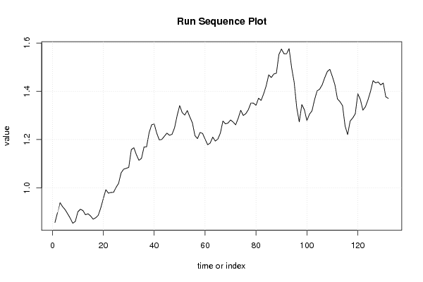
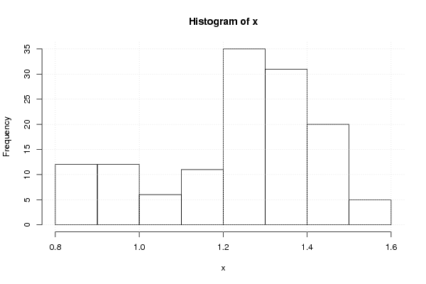
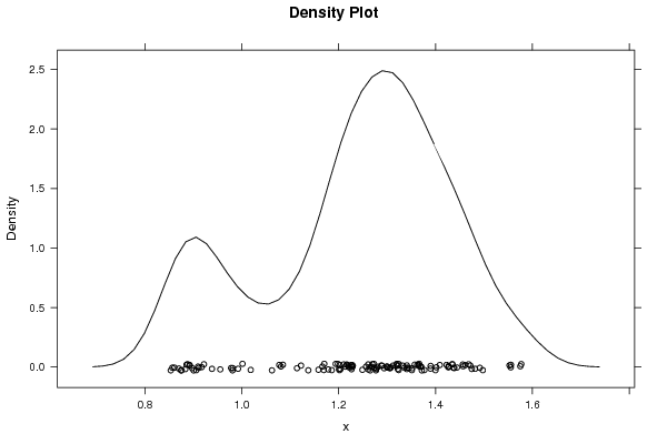
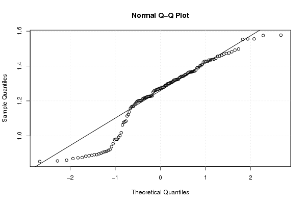
| Title produced by software | Univariate Explorative Data Analysis | ||||||||||||||||||||||||||||||||||||||||||||||||||||
| Date of computation | Mon, 19 Dec 2011 06:44:59 -0500 | ||||||||||||||||||||||||||||||||||||||||||||||||||||
| Cite this page as follows | Statistical Computations at FreeStatistics.org, Office for Research Development and Education, URL https://freestatistics.org/blog/index.php?v=date/2011/Dec/19/t132429514190umhf7m4ugowy1.htm/, Retrieved Tue, 28 Jul 2026 04:49:56 +0000 | ||||||||||||||||||||||||||||||||||||||||||||||||||||
| Statistical Computations at FreeStatistics.org, Office for Research Development and Education, URL https://freestatistics.org/blog/index.php?pk=157290, Retrieved Tue, 28 Jul 2026 04:49:56 +0000 | |||||||||||||||||||||||||||||||||||||||||||||||||||||
| QR Codes: | |||||||||||||||||||||||||||||||||||||||||||||||||||||
|
| |||||||||||||||||||||||||||||||||||||||||||||||||||||
| Original text written by user: | |||||||||||||||||||||||||||||||||||||||||||||||||||||
| IsPrivate? | No (this computation is public) | ||||||||||||||||||||||||||||||||||||||||||||||||||||
| User-defined keywords | |||||||||||||||||||||||||||||||||||||||||||||||||||||
| Estimated Impact | 452 | ||||||||||||||||||||||||||||||||||||||||||||||||||||
Tree of Dependent Computations | |||||||||||||||||||||||||||||||||||||||||||||||||||||
| Family? (F = Feedback message, R = changed R code, M = changed R Module, P = changed Parameters, D = changed Data) | |||||||||||||||||||||||||||||||||||||||||||||||||||||
| - [Univariate Data Series] [] [2009-12-18 13:45:47] [4409a44d89cea4fe559b38f99bc8a66c] - RMPD [Univariate Explorative Data Analysis] [Paper univariate EDA] [2011-12-19 11:44:59] [3627de22d386f4cb93d383ef7c1ade7f] [Current] - R [Univariate Explorative Data Analysis] [Paper univariate ...] [2011-12-19 11:53:03] [aba4febe8a2e49e81bdc61a6c01f5c21] - D [Univariate Explorative Data Analysis] [Paper univariate ...] [2011-12-19 11:54:57] [aba4febe8a2e49e81bdc61a6c01f5c21] - D [Univariate Explorative Data Analysis] [Paper univariate ...] [2011-12-19 11:56:33] [aba4febe8a2e49e81bdc61a6c01f5c21] - RM D [Kendall tau Correlation Matrix] [Paper Pearson Cor...] [2011-12-19 12:01:08] [aba4febe8a2e49e81bdc61a6c01f5c21] - RM D [Kendall tau Correlation Matrix] [Paper Kendall Tau...] [2011-12-19 12:08:43] [aba4febe8a2e49e81bdc61a6c01f5c21] | |||||||||||||||||||||||||||||||||||||||||||||||||||||
| Feedback Forum | |||||||||||||||||||||||||||||||||||||||||||||||||||||
Post a new message | |||||||||||||||||||||||||||||||||||||||||||||||||||||
Dataset | |||||||||||||||||||||||||||||||||||||||||||||||||||||
| Dataseries X: | |||||||||||||||||||||||||||||||||||||||||||||||||||||
0.8564 0.8973 0.9383 0.9217 0.9095 0.892 0.8742 0.8532 0.8607 0.9005 0.9111 0.9059 0.8883 0.8924 0.8833 0.87 0.8758 0.8858 0.917 0.9554 0.9922 0.9778 0.9808 0.9811 1.0014 1.0183 1.0622 1.0773 1.0807 1.0848 1.1582 1.1663 1.1372 1.1139 1.1222 1.1692 1.1702 1.2286 1.2613 1.2646 1.2262 1.1985 1.2007 1.2138 1.2266 1.2176 1.2218 1.249 1.2991 1.3408 1.3119 1.3014 1.3201 1.2938 1.2694 1.2165 1.2037 1.2292 1.2256 1.2015 1.1786 1.1856 1.2103 1.1938 1.202 1.2271 1.277 1.265 1.2684 1.2811 1.2727 1.2611 1.2881 1.3213 1.2999 1.3074 1.3242 1.3516 1.3511 1.3419 1.3716 1.3622 1.3896 1.4227 1.4684 1.457 1.4718 1.4748 1.5527 1.575 1.5557 1.5553 1.577 1.4975 1.437 1.3322 1.2732 1.3449 1.3239 1.2785 1.305 1.319 1.365 1.4016 1.4088 1.4268 1.4562 1.4816 1.4914 1.4614 1.4272 1.3686 1.3569 1.3406 1.2565 1.2208 1.277 1.2894 1.3067 1.3898 1.3661 1.322 1.336 1.3649 1.3999 1.4442 1.4349 1.4388 1.4264 1.4343 1.377 1.3706 | |||||||||||||||||||||||||||||||||||||||||||||||||||||
Tables (Output of Computation) | |||||||||||||||||||||||||||||||||||||||||||||||||||||
| |||||||||||||||||||||||||||||||||||||||||||||||||||||
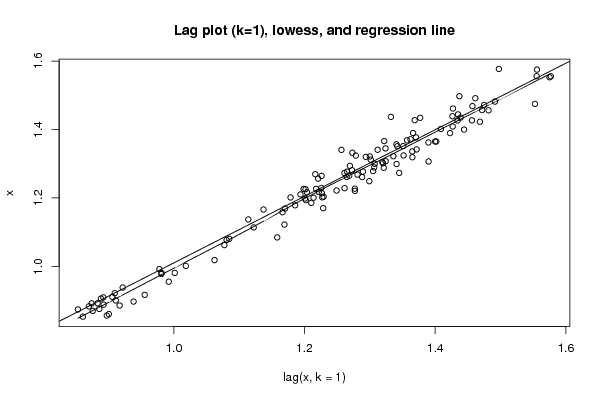
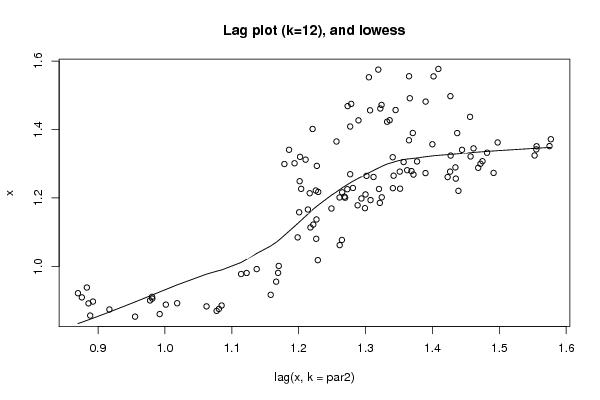
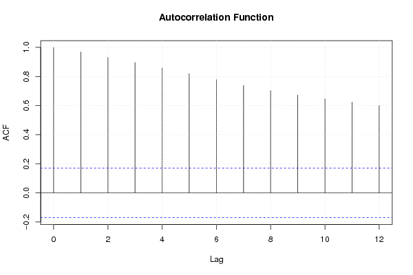
Figures (Output of Computation) | |||||||||||||||||||||||||||||||||||||||||||||||||||||
Input Parameters & R Code | |||||||||||||||||||||||||||||||||||||||||||||||||||||
| Parameters (Session): | |||||||||||||||||||||||||||||||||||||||||||||||||||||
| par1 = 0 ; par2 = 12 ; | |||||||||||||||||||||||||||||||||||||||||||||||||||||
| Parameters (R input): | |||||||||||||||||||||||||||||||||||||||||||||||||||||
| par1 = 0 ; par2 = 12 ; | |||||||||||||||||||||||||||||||||||||||||||||||||||||
| R code (references can be found in the software module): | |||||||||||||||||||||||||||||||||||||||||||||||||||||
par1 <- as.numeric(par1) | |||||||||||||||||||||||||||||||||||||||||||||||||||||