\begin{tabular}{lllllllll}
\hline
Summary of computational transaction \tabularnewline
Raw Input & view raw input (R code)  \tabularnewline
Raw Output & view raw output of R engine  \tabularnewline
Computing time & 2 seconds \tabularnewline
R Server & 'Gwilym Jenkins' @ jenkins.wessa.net \tabularnewline
\hline
\end{tabular}
%Source: https://freestatistics.org/blog/index.php?pk=232512&T=0
[TABLE]
[ROW][C]Summary of computational transaction[/C][/ROW]
[ROW][C]Raw Input[/C][C]view raw input (R code) [/C][/ROW]
[ROW][C]Raw Output[/C][C]view raw output of R engine [/C][/ROW]
[ROW][C]Computing time[/C][C]2 seconds[/C][/ROW]
[ROW][C]R Server[/C][C]'Gwilym Jenkins' @ jenkins.wessa.net[/C][/ROW]
[/TABLE]
Source: https://freestatistics.org/blog/index.php?pk=232512&T=0
If you paste this QR Code into your document, anyone with a smartphone or tablet will be able to scan it and view this table in a browser.
If you paste this QR Code into your document, anyone with a smartphone or tablet will be able to scan it and view this table in a browser.
If you paste this QR Code into your document, anyone with a smartphone or tablet will be able to scan it and view this table in a browser.
If you paste this QR Code into your document, anyone with a smartphone or tablet will be able to scan it and view this table in a browser.
If you paste this QR Code into your document, anyone with a smartphone or tablet will be able to scan it and view this table in a browser.
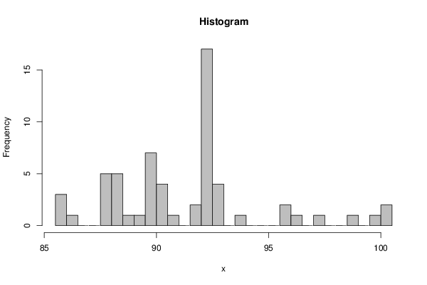
| Frequency Table (Histogram) | | Bins | Midpoint | Abs. Frequency | Rel. Frequency | Cumul. Rel. Freq. | Density | | [85.5,86[ | 85.75 | 3 | 0.05 | 0.05 | 0.1 | | [86,86.5[ | 86.25 | 1 | 0.016667 | 0.066667 | 0.033333 | | [86.5,87[ | 86.75 | 0 | 0 | 0.066667 | 0 | | [87,87.5[ | 87.25 | 0 | 0 | 0.066667 | 0 | | [87.5,88[ | 87.75 | 5 | 0.083333 | 0.15 | 0.166667 | | [88,88.5[ | 88.25 | 5 | 0.083333 | 0.233333 | 0.166667 | | [88.5,89[ | 88.75 | 1 | 0.016667 | 0.25 | 0.033333 | | [89,89.5[ | 89.25 | 1 | 0.016667 | 0.266667 | 0.033333 | | [89.5,90[ | 89.75 | 7 | 0.116667 | 0.383333 | 0.233333 | | [90,90.5[ | 90.25 | 4 | 0.066667 | 0.45 | 0.133333 | | [90.5,91[ | 90.75 | 1 | 0.016667 | 0.466667 | 0.033333 | | [91,91.5[ | 91.25 | 0 | 0 | 0.466667 | 0 | | [91.5,92[ | 91.75 | 2 | 0.033333 | 0.5 | 0.066667 | | [92,92.5[ | 92.25 | 17 | 0.283333 | 0.783333 | 0.566667 | | [92.5,93[ | 92.75 | 4 | 0.066667 | 0.85 | 0.133333 | | [93,93.5[ | 93.25 | 0 | 0 | 0.85 | 0 | | [93.5,94[ | 93.75 | 1 | 0.016667 | 0.866667 | 0.033333 | | [94,94.5[ | 94.25 | 0 | 0 | 0.866667 | 0 | | [94.5,95[ | 94.75 | 0 | 0 | 0.866667 | 0 | | [95,95.5[ | 95.25 | 0 | 0 | 0.866667 | 0 | | [95.5,96[ | 95.75 | 2 | 0.033333 | 0.9 | 0.066667 | | [96,96.5[ | 96.25 | 1 | 0.016667 | 0.916667 | 0.033333 | | [96.5,97[ | 96.75 | 0 | 0 | 0.916667 | 0 | | [97,97.5[ | 97.25 | 1 | 0.016667 | 0.933333 | 0.033333 | | [97.5,98[ | 97.75 | 0 | 0 | 0.933333 | 0 | | [98,98.5[ | 98.25 | 0 | 0 | 0.933333 | 0 | | [98.5,99[ | 98.75 | 1 | 0.016667 | 0.95 | 0.033333 | | [99,99.5[ | 99.25 | 0 | 0 | 0.95 | 0 | | [99.5,100[ | 99.75 | 1 | 0.016667 | 0.966667 | 0.033333 | | [100,100.5] | 100.25 | 2 | 0.033333 | 1 | 0.066667 |
\begin{tabular}{lllllllll}
\hline
Frequency Table (Histogram) \tabularnewline
Bins & Midpoint & Abs. Frequency & Rel. Frequency & Cumul. Rel. Freq. & Density \tabularnewline
[85.5,86[ & 85.75 & 3 & 0.05 & 0.05 & 0.1 \tabularnewline
[86,86.5[ & 86.25 & 1 & 0.016667 & 0.066667 & 0.033333 \tabularnewline
[86.5,87[ & 86.75 & 0 & 0 & 0.066667 & 0 \tabularnewline
[87,87.5[ & 87.25 & 0 & 0 & 0.066667 & 0 \tabularnewline
[87.5,88[ & 87.75 & 5 & 0.083333 & 0.15 & 0.166667 \tabularnewline
[88,88.5[ & 88.25 & 5 & 0.083333 & 0.233333 & 0.166667 \tabularnewline
[88.5,89[ & 88.75 & 1 & 0.016667 & 0.25 & 0.033333 \tabularnewline
[89,89.5[ & 89.25 & 1 & 0.016667 & 0.266667 & 0.033333 \tabularnewline
[89.5,90[ & 89.75 & 7 & 0.116667 & 0.383333 & 0.233333 \tabularnewline
[90,90.5[ & 90.25 & 4 & 0.066667 & 0.45 & 0.133333 \tabularnewline
[90.5,91[ & 90.75 & 1 & 0.016667 & 0.466667 & 0.033333 \tabularnewline
[91,91.5[ & 91.25 & 0 & 0 & 0.466667 & 0 \tabularnewline
[91.5,92[ & 91.75 & 2 & 0.033333 & 0.5 & 0.066667 \tabularnewline
[92,92.5[ & 92.25 & 17 & 0.283333 & 0.783333 & 0.566667 \tabularnewline
[92.5,93[ & 92.75 & 4 & 0.066667 & 0.85 & 0.133333 \tabularnewline
[93,93.5[ & 93.25 & 0 & 0 & 0.85 & 0 \tabularnewline
[93.5,94[ & 93.75 & 1 & 0.016667 & 0.866667 & 0.033333 \tabularnewline
[94,94.5[ & 94.25 & 0 & 0 & 0.866667 & 0 \tabularnewline
[94.5,95[ & 94.75 & 0 & 0 & 0.866667 & 0 \tabularnewline
[95,95.5[ & 95.25 & 0 & 0 & 0.866667 & 0 \tabularnewline
[95.5,96[ & 95.75 & 2 & 0.033333 & 0.9 & 0.066667 \tabularnewline
[96,96.5[ & 96.25 & 1 & 0.016667 & 0.916667 & 0.033333 \tabularnewline
[96.5,97[ & 96.75 & 0 & 0 & 0.916667 & 0 \tabularnewline
[97,97.5[ & 97.25 & 1 & 0.016667 & 0.933333 & 0.033333 \tabularnewline
[97.5,98[ & 97.75 & 0 & 0 & 0.933333 & 0 \tabularnewline
[98,98.5[ & 98.25 & 0 & 0 & 0.933333 & 0 \tabularnewline
[98.5,99[ & 98.75 & 1 & 0.016667 & 0.95 & 0.033333 \tabularnewline
[99,99.5[ & 99.25 & 0 & 0 & 0.95 & 0 \tabularnewline
[99.5,100[ & 99.75 & 1 & 0.016667 & 0.966667 & 0.033333 \tabularnewline
[100,100.5] & 100.25 & 2 & 0.033333 & 1 & 0.066667 \tabularnewline
\hline
\end{tabular}
%Source: https://freestatistics.org/blog/index.php?pk=232512&T=1
[TABLE]
[ROW][C]Frequency Table (Histogram)[/C][/ROW]
[ROW][C]Bins[/C][C]Midpoint[/C][C]Abs. Frequency[/C][C]Rel. Frequency[/C][C]Cumul. Rel. Freq.[/C][C]Density[/C][/ROW]
[ROW][C][85.5,86[[/C][C]85.75[/C][C]3[/C][C]0.05[/C][C]0.05[/C][C]0.1[/C][/ROW]
[ROW][C][86,86.5[[/C][C]86.25[/C][C]1[/C][C]0.016667[/C][C]0.066667[/C][C]0.033333[/C][/ROW]
[ROW][C][86.5,87[[/C][C]86.75[/C][C]0[/C][C]0[/C][C]0.066667[/C][C]0[/C][/ROW]
[ROW][C][87,87.5[[/C][C]87.25[/C][C]0[/C][C]0[/C][C]0.066667[/C][C]0[/C][/ROW]
[ROW][C][87.5,88[[/C][C]87.75[/C][C]5[/C][C]0.083333[/C][C]0.15[/C][C]0.166667[/C][/ROW]
[ROW][C][88,88.5[[/C][C]88.25[/C][C]5[/C][C]0.083333[/C][C]0.233333[/C][C]0.166667[/C][/ROW]
[ROW][C][88.5,89[[/C][C]88.75[/C][C]1[/C][C]0.016667[/C][C]0.25[/C][C]0.033333[/C][/ROW]
[ROW][C][89,89.5[[/C][C]89.25[/C][C]1[/C][C]0.016667[/C][C]0.266667[/C][C]0.033333[/C][/ROW]
[ROW][C][89.5,90[[/C][C]89.75[/C][C]7[/C][C]0.116667[/C][C]0.383333[/C][C]0.233333[/C][/ROW]
[ROW][C][90,90.5[[/C][C]90.25[/C][C]4[/C][C]0.066667[/C][C]0.45[/C][C]0.133333[/C][/ROW]
[ROW][C][90.5,91[[/C][C]90.75[/C][C]1[/C][C]0.016667[/C][C]0.466667[/C][C]0.033333[/C][/ROW]
[ROW][C][91,91.5[[/C][C]91.25[/C][C]0[/C][C]0[/C][C]0.466667[/C][C]0[/C][/ROW]
[ROW][C][91.5,92[[/C][C]91.75[/C][C]2[/C][C]0.033333[/C][C]0.5[/C][C]0.066667[/C][/ROW]
[ROW][C][92,92.5[[/C][C]92.25[/C][C]17[/C][C]0.283333[/C][C]0.783333[/C][C]0.566667[/C][/ROW]
[ROW][C][92.5,93[[/C][C]92.75[/C][C]4[/C][C]0.066667[/C][C]0.85[/C][C]0.133333[/C][/ROW]
[ROW][C][93,93.5[[/C][C]93.25[/C][C]0[/C][C]0[/C][C]0.85[/C][C]0[/C][/ROW]
[ROW][C][93.5,94[[/C][C]93.75[/C][C]1[/C][C]0.016667[/C][C]0.866667[/C][C]0.033333[/C][/ROW]
[ROW][C][94,94.5[[/C][C]94.25[/C][C]0[/C][C]0[/C][C]0.866667[/C][C]0[/C][/ROW]
[ROW][C][94.5,95[[/C][C]94.75[/C][C]0[/C][C]0[/C][C]0.866667[/C][C]0[/C][/ROW]
[ROW][C][95,95.5[[/C][C]95.25[/C][C]0[/C][C]0[/C][C]0.866667[/C][C]0[/C][/ROW]
[ROW][C][95.5,96[[/C][C]95.75[/C][C]2[/C][C]0.033333[/C][C]0.9[/C][C]0.066667[/C][/ROW]
[ROW][C][96,96.5[[/C][C]96.25[/C][C]1[/C][C]0.016667[/C][C]0.916667[/C][C]0.033333[/C][/ROW]
[ROW][C][96.5,97[[/C][C]96.75[/C][C]0[/C][C]0[/C][C]0.916667[/C][C]0[/C][/ROW]
[ROW][C][97,97.5[[/C][C]97.25[/C][C]1[/C][C]0.016667[/C][C]0.933333[/C][C]0.033333[/C][/ROW]
[ROW][C][97.5,98[[/C][C]97.75[/C][C]0[/C][C]0[/C][C]0.933333[/C][C]0[/C][/ROW]
[ROW][C][98,98.5[[/C][C]98.25[/C][C]0[/C][C]0[/C][C]0.933333[/C][C]0[/C][/ROW]
[ROW][C][98.5,99[[/C][C]98.75[/C][C]1[/C][C]0.016667[/C][C]0.95[/C][C]0.033333[/C][/ROW]
[ROW][C][99,99.5[[/C][C]99.25[/C][C]0[/C][C]0[/C][C]0.95[/C][C]0[/C][/ROW]
[ROW][C][99.5,100[[/C][C]99.75[/C][C]1[/C][C]0.016667[/C][C]0.966667[/C][C]0.033333[/C][/ROW]
[ROW][C][100,100.5][/C][C]100.25[/C][C]2[/C][C]0.033333[/C][C]1[/C][C]0.066667[/C][/ROW]
[/TABLE]
Source: https://freestatistics.org/blog/index.php?pk=232512&T=1
Globally Unique Identifier (entire table): ba.freestatistics.org/blog/index.php?pk=232512&T=1
As an alternative you can also use a QR Code:
The GUIDs for individual cells are displayed in the table below:
| Frequency Table (Histogram) | | Bins | Midpoint | Abs. Frequency | Rel. Frequency | Cumul. Rel. Freq. | Density | | [85.5,86[ | 85.75 | 3 | 0.05 | 0.05 | 0.1 | | [86,86.5[ | 86.25 | 1 | 0.016667 | 0.066667 | 0.033333 | | [86.5,87[ | 86.75 | 0 | 0 | 0.066667 | 0 | | [87,87.5[ | 87.25 | 0 | 0 | 0.066667 | 0 | | [87.5,88[ | 87.75 | 5 | 0.083333 | 0.15 | 0.166667 | | [88,88.5[ | 88.25 | 5 | 0.083333 | 0.233333 | 0.166667 | | [88.5,89[ | 88.75 | 1 | 0.016667 | 0.25 | 0.033333 | | [89,89.5[ | 89.25 | 1 | 0.016667 | 0.266667 | 0.033333 | | [89.5,90[ | 89.75 | 7 | 0.116667 | 0.383333 | 0.233333 | | [90,90.5[ | 90.25 | 4 | 0.066667 | 0.45 | 0.133333 | | [90.5,91[ | 90.75 | 1 | 0.016667 | 0.466667 | 0.033333 | | [91,91.5[ | 91.25 | 0 | 0 | 0.466667 | 0 | | [91.5,92[ | 91.75 | 2 | 0.033333 | 0.5 | 0.066667 | | [92,92.5[ | 92.25 | 17 | 0.283333 | 0.783333 | 0.566667 | | [92.5,93[ | 92.75 | 4 | 0.066667 | 0.85 | 0.133333 | | [93,93.5[ | 93.25 | 0 | 0 | 0.85 | 0 | | [93.5,94[ | 93.75 | 1 | 0.016667 | 0.866667 | 0.033333 | | [94,94.5[ | 94.25 | 0 | 0 | 0.866667 | 0 | | [94.5,95[ | 94.75 | 0 | 0 | 0.866667 | 0 | | [95,95.5[ | 95.25 | 0 | 0 | 0.866667 | 0 | | [95.5,96[ | 95.75 | 2 | 0.033333 | 0.9 | 0.066667 | | [96,96.5[ | 96.25 | 1 | 0.016667 | 0.916667 | 0.033333 | | [96.5,97[ | 96.75 | 0 | 0 | 0.916667 | 0 | | [97,97.5[ | 97.25 | 1 | 0.016667 | 0.933333 | 0.033333 | | [97.5,98[ | 97.75 | 0 | 0 | 0.933333 | 0 | | [98,98.5[ | 98.25 | 0 | 0 | 0.933333 | 0 | | [98.5,99[ | 98.75 | 1 | 0.016667 | 0.95 | 0.033333 | | [99,99.5[ | 99.25 | 0 | 0 | 0.95 | 0 | | [99.5,100[ | 99.75 | 1 | 0.016667 | 0.966667 | 0.033333 | | [100,100.5] | 100.25 | 2 | 0.033333 | 1 | 0.066667 |
If you paste this QR Code into your document, anyone with a smartphone or tablet will be able to scan it and view this table in a browser.
If you paste this QR Code into your document, anyone with a smartphone or tablet will be able to scan it and view this table in a browser.
If you paste this QR Code into your document, anyone with a smartphone or tablet will be able to scan it and view this table in a browser.
If you paste this QR Code into your document, anyone with a smartphone or tablet will be able to scan it and view this table in a browser.
If you paste this QR Code into your document, anyone with a smartphone or tablet will be able to scan it and view this table in a browser.
|