Repository of Reproducible Computations

Free Statistics

of Irreproducible Research!

Author's title

Author

*The author of this computation has been verified*

R Software Module

rwasp_fitdistrnorm.wasp

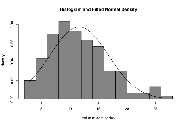
Title produced by software

ML Fitting and QQ Plot- Normal Distribution

Date of computation

Mon, 28 Sep 2015 11:39:26 +0100

Cite this page as follows

Statistical Computations at FreeStatistics.org, Office for Research Development and Education, URL https://freestatistics.org/blog/index.php?v=date/2015/Sep/28/t1443436784jsihgsh1nfzge2b.htm/, Retrieved Thu, 09 May 2024 02:47:32 +0000

Statistical Computations at FreeStatistics.org, Office for Research Development and Education, URL https://freestatistics.org/blog/index.php?pk=280705, Retrieved Thu, 09 May 2024 02:47:32 +0000

QR Codes:

Paste this QR Code to cite your computation.

Original text written by user:

IsPrivate?

No (this computation is public)

User-defined keywords

Estimated Impact

707

Family? (F = Feedback message, R = changed R code, M = changed R Module, P = changed Parameters, D = changed Data)

-       [ML Fitting and QQ Plot- Normal Distribution] [] [2015-09-28 10:39:26] [63a9f0ea7bb98050796b649e85481845] [Current]
- RMPD    [Histogram] [Frequency Plot of...] [2016-10-22 09:37:48] [febbe70567d8817ee05b7c8fe7dbe7a8] 
- RMPD    [Histogram] [ Frequency Plot o...] [2016-10-22 10:04:51] [febbe70567d8817ee05b7c8fe7dbe7a8] 

Feedback Forum

Post a new message

Dataseries X:

Download CSV

Histogram

Boxplots

7.159583212
8.720190863
11.35012188
11.19985172
8.886930789
12.32716938
12.18248575
19.90570486
9.138870744
2.823345199
6.697273807
19.14246314
8.52501489
15.46933257
11.89887459
14.11970083
9.759524117
10.72777406
24.84064617
18.81108017
13.36224609
14.42070356
13.35225123
9.768458244
13.48950731
7.453982835
13.98274836
20.96990106
22.82593137
8.526208745
17.09784219
16.32109031
11.50223142
25.49243141
13.02274287
11.00454638
5.201297025
6.24602302
5.222681151
8.649211832
4.99646075
7.766766126
6.414759189
7.880830486
10.05880371
11.16783112
4.097158679
8.654343733
12.08969867
15.69307678
11.15843137
5.845182723
4.531612623
11.62969358
9.436199568
6.464241484
6.487618541
25.1230787
13.51578068
19.61654091
13.32488597
21.8441133
15.0758351
10.77914539
3.771562069
17.38382154
13.49752596
2.716158175
9.810291912
10.94698801
5.155930406
9.23315008
12.71345045
10.08532187
10.97007548
13.658909
12.82263869
24.0289767
6.260649968
18.13338307
14.57175459
8.144770398
8.727422622
15.09633963
6.621862669
18.92080233
9.820085897
8.566240811
14.31947202
13.29848355
9.073755521
11.19352288
3.80888864
14.55315591
26.62180318
8.543507246
8.123577983
17.62154625
6.478910673
12.59200449
11.68188403
15.43755005
7.861997091
15.84800609
7.540903857
10.08266066
7.824972906
16.7097823
19.8880974
5.294059094
11.34614334
9.241176097
6.78288623
7.858918189
8.421923427
11.47350713
4.175198586
6.695712845
5.65850228
14.90524411
6.755921852
17.29503554
13.34590912
5.402551189
7.456145495
14.13581614
14.15087234
3.804524754
19.63104972
10.28781088
17.26946999
11.01478839
15.21572044
9.871093246
8.82819689
3.587580869
17.1331504
12.50638353
16.02662305
5.233040184
9.426048176
6.808302128
10.2280652
12.28629292
22.90115925
19.02333532
14.11860564
14.32178369
9.575536885
5.449874123

Summary of computational transaction
Raw Input	view raw input (R code)
Raw Output	view raw output of R engine
Computing time	4 seconds
R Server	'George Udny Yule' @ yule.wessa.net

\begin{tabular}{lllllllll}
\hline
Summary of computational transaction \tabularnewline
Raw Input & view raw input (R code)  \tabularnewline
Raw Output & view raw output of R engine  \tabularnewline
Computing time & 4 seconds \tabularnewline
R Server & 'George Udny Yule' @ yule.wessa.net \tabularnewline
\hline
\end{tabular}
%Source: https://freestatistics.org/blog/index.php?pk=280705&T=0

[TABLE]
[ROW][C]Summary of computational transaction[/C][/ROW]
[ROW][C]Raw Input[/C][C]view raw input (R code) [/C][/ROW]
[ROW][C]Raw Output[/C][C]view raw output of R engine [/C][/ROW]
[ROW][C]Computing time[/C][C]4 seconds[/C][/ROW]
[ROW][C]R Server[/C][C]'George Udny Yule' @ yule.wessa.net[/C][/ROW]
[/TABLE]
Source: https://freestatistics.org/blog/index.php?pk=280705&T=0

Globally Unique Identifier (entire table): ba.freestatistics.org/blog/index.php?pk=280705&T=0

As an alternative you can also use a QR Code:

The GUIDs for individual cells are displayed in the table below:

Summary of computational transaction
Raw Input	view raw input (R code)
Raw Output	view raw output of R engine
Computing time	4 seconds
R Server	'George Udny Yule' @ yule.wessa.net

Parameter	Estimated Value	Standard Deviation
mean	11.6063774537867	0.420644606327626
standard deviation	5.15182324278294	0.29744065360381

\begin{tabular}{lllllllll}
\hline
Parameter & Estimated Value & Standard Deviation \tabularnewline
mean & 11.6063774537867 & 0.420644606327626 \tabularnewline
standard deviation & 5.15182324278294 & 0.29744065360381 \tabularnewline
\hline
\end{tabular}
%Source: https://freestatistics.org/blog/index.php?pk=280705&T=1

[TABLE]
[ROW][C]Parameter[/C][C]Estimated Value[/C][C]Standard Deviation[/C][/ROW]
[ROW][C]mean[/C][C]11.6063774537867[/C][C]0.420644606327626[/C][/ROW]
[ROW][C]standard deviation[/C][C]5.15182324278294[/C][C]0.29744065360381[/C][/ROW]
[/TABLE]
Source: https://freestatistics.org/blog/index.php?pk=280705&T=1

Globally Unique Identifier (entire table): ba.freestatistics.org/blog/index.php?pk=280705&T=1

As an alternative you can also use a QR Code:

The GUIDs for individual cells are displayed in the table below:

Parameter	Estimated Value	Standard Deviation
mean	11.6063774537867	0.420644606327626
standard deviation	5.15182324278294	0.29744065360381

Figure 1

PNG link

Postscript link

PDF link

Figure 2

PNG link

Postscript link

PDF link

Parameters (Session):

par1 = 8 ; par2 = 0 ;

Parameters (R input):

par1 = 8 ; par2 = 0 ;

R code (references can be found in the software module):

library(MASS)
library(car)
par1 <- as.numeric(par1)
if (par2 == '0') par2 = 'Sturges' else par2 <- as.numeric(par2)
x <- as.ts(x) #otherwise the fitdistr function does not work properly
r <- fitdistr(x,'normal')
r
bitmap(file='test1.png')
myhist<-hist(x,col=par1,breaks=par2,main=main,ylab=ylab,xlab=xlab,freq=F)
curve(1/(r$estimate[2]*sqrt(2*pi))*exp(-1/2*((x-r$estimate[1])/r$estimate[2])^2),min(x),max(x),add=T)
dev.off()
bitmap(file='test3.png')
qqPlot(x,dist='norm',main='QQ plot (Normal) with confidence intervals')
grid()
dev.off()
load(file='createtable')
a<-table.start()
a<-table.row.start(a)
a<-table.element(a,'Parameter',1,TRUE)
a<-table.element(a,'Estimated Value',1,TRUE)
a<-table.element(a,'Standard Deviation',1,TRUE)
a<-table.row.end(a)
a<-table.row.start(a)
a<-table.element(a,'mean',header=TRUE)
a<-table.element(a,r$estimate[1])
a<-table.element(a,r$sd[1])
a<-table.row.end(a)
a<-table.row.start(a)
a<-table.element(a,'standard deviation',header=TRUE)
a<-table.element(a,r$estimate[2])
a<-table.element(a,r$sd[2])
a<-table.row.end(a)
a<-table.end(a)
table.save(a,file='mytable.tab')

Free Statistics

Description of Statistical Computation

Tree of Dependent Computations

Dataset

Tables (Output of Computation)

Figures (Output of Computation)

Input Parameters & R Code