Free Statistics
of Irreproducible Research!
Description of Statistical Computation | |||||||||||||||||||||
|---|---|---|---|---|---|---|---|---|---|---|---|---|---|---|---|---|---|---|---|---|---|
| Author's title | |||||||||||||||||||||
| Author | *Unverified author* | ||||||||||||||||||||
| R Software Module | rwasp_sdplot.wasp | ||||||||||||||||||||
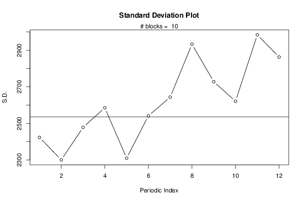
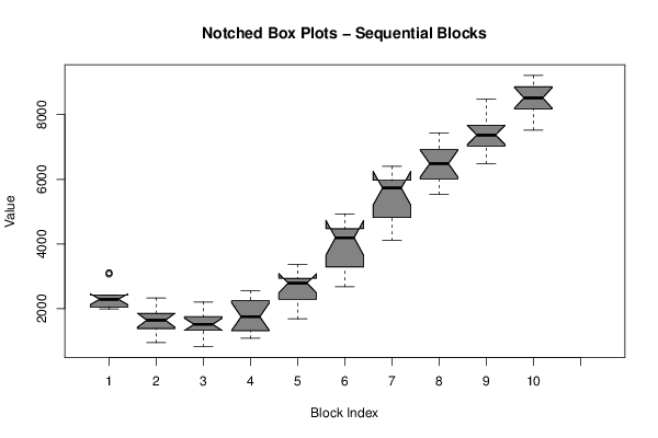
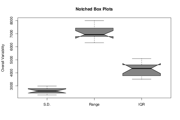
| Title produced by software | Standard Deviation Plot | ||||||||||||||||||||
| Date of computation | Tue, 09 Aug 2016 11:45:04 +0100 | ||||||||||||||||||||
| Cite this page as follows | Statistical Computations at FreeStatistics.org, Office for Research Development and Education, URL https://freestatistics.org/blog/index.php?v=date/2016/Aug/09/t14707395406bdzae5n3867h9z.htm/, Retrieved Tue, 19 May 2026 13:27:18 +0000 | ||||||||||||||||||||
| Statistical Computations at FreeStatistics.org, Office for Research Development and Education, URL https://freestatistics.org/blog/index.php?pk=296131, Retrieved Tue, 19 May 2026 13:27:18 +0000 | |||||||||||||||||||||
| QR Codes: | |||||||||||||||||||||
|
| |||||||||||||||||||||
| Original text written by user: | |||||||||||||||||||||
| IsPrivate? | No (this computation is public) | ||||||||||||||||||||
| User-defined keywords | |||||||||||||||||||||
| Estimated Impact | 391 | ||||||||||||||||||||
Tree of Dependent Computations | |||||||||||||||||||||
| Family? (F = Feedback message, R = changed R code, M = changed R Module, P = changed Parameters, D = changed Data) | |||||||||||||||||||||
| - [Univariate Data Series] [omzet lego technique] [2016-08-08 19:25:41] [74be16979710d4c4e7c6647856088456] - RMPD [Harrell-Davis Quantiles] [Harrel-Davis quan...] [2016-08-08 22:07:37] [4c392b130fccc63297597dd6ffb6df17] - RM D [(Partial) Autocorrelation Function] [partial autocorre...] [2016-08-09 10:29:16] [4c392b130fccc63297597dd6ffb6df17] - RM D [Standard Deviation Plot] [standard deviatio...] [2016-08-09 10:45:04] [d7adcc7732e5b057da1b42af54844e1a] [Current] | |||||||||||||||||||||
| Feedback Forum | |||||||||||||||||||||
Post a new message | |||||||||||||||||||||
Dataset | |||||||||||||||||||||
| Dataseries X: | |||||||||||||||||||||
2421.21 2378.63 2336.00 2250.79 3113.00 3070.38 2421.21 1990.13 2032.71 2032.71 2075.33 2165.17 1904.92 1644.25 1430.79 1430.79 2250.79 2336.00 1686.83 952.46 1340.96 1340.96 1644.25 1819.29 1776.67 1340.96 1559.04 1473.42 2207.79 2032.71 1340.96 824.25 1298.33 1430.79 1559.04 1729.46 1383.54 1084.92 1213.17 1255.75 2378.63 2378.63 1729.46 1644.25 1904.92 1776.67 2122.58 2553.67 2639.29 2032.71 1861.88 1686.83 2856.96 2942.58 2724.50 2942.58 2899.54 2553.67 2942.58 3373.67 3548.71 3027.79 2681.88 2942.58 4065.42 4411.33 4326.13 4496.50 4453.92 4022.83 4757.21 4932.25 5188.29 4411.33 4108.04 4453.92 5278.13 6012.50 5837.46 5837.46 5923.08 5624.00 6401.42 6401.42 6268.96 5534.17 5666.63 5752.25 6315.79 7050.17 6529.21 6789.92 6571.83 6444.00 7439.08 7221.00 6917.71 6486.63 6917.71 7135.79 7396.04 7741.92 7396.04 7609.50 7349.21 7306.63 8386.88 8476.71 8130.83 7524.29 8041.00 8258.67 8519.33 8907.83 8519.33 8822.63 8690.17 8216.04 9211.08 9211.08 | |||||||||||||||||||||
Tables (Output of Computation) | |||||||||||||||||||||
| |||||||||||||||||||||
Figures (Output of Computation) | |||||||||||||||||||||
Input Parameters & R Code | |||||||||||||||||||||
| Parameters (Session): | |||||||||||||||||||||
| Parameters (R input): | |||||||||||||||||||||
| par1 = 12 ; | |||||||||||||||||||||
| R code (references can be found in the software module): | |||||||||||||||||||||
par1 <- as.numeric(par1) | |||||||||||||||||||||