Free Statistics
of Irreproducible Research!
Description of Statistical Computation | |||||||||||||||||||||||||||||||||||||||||||||||||||||||||||||||||||||||||||||||||||||||||||||||||||||||||||||||||||||||||||||||||||||||||||||||||||||||||
|---|---|---|---|---|---|---|---|---|---|---|---|---|---|---|---|---|---|---|---|---|---|---|---|---|---|---|---|---|---|---|---|---|---|---|---|---|---|---|---|---|---|---|---|---|---|---|---|---|---|---|---|---|---|---|---|---|---|---|---|---|---|---|---|---|---|---|---|---|---|---|---|---|---|---|---|---|---|---|---|---|---|---|---|---|---|---|---|---|---|---|---|---|---|---|---|---|---|---|---|---|---|---|---|---|---|---|---|---|---|---|---|---|---|---|---|---|---|---|---|---|---|---|---|---|---|---|---|---|---|---|---|---|---|---|---|---|---|---|---|---|---|---|---|---|---|---|---|---|---|---|---|---|---|
| Author's title | |||||||||||||||||||||||||||||||||||||||||||||||||||||||||||||||||||||||||||||||||||||||||||||||||||||||||||||||||||||||||||||||||||||||||||||||||||||||||
| Author | *The author of this computation has been verified* | ||||||||||||||||||||||||||||||||||||||||||||||||||||||||||||||||||||||||||||||||||||||||||||||||||||||||||||||||||||||||||||||||||||||||||||||||||||||||
| R Software Module | rwasp_histogram.wasp | ||||||||||||||||||||||||||||||||||||||||||||||||||||||||||||||||||||||||||||||||||||||||||||||||||||||||||||||||||||||||||||||||||||||||||||||||||||||||
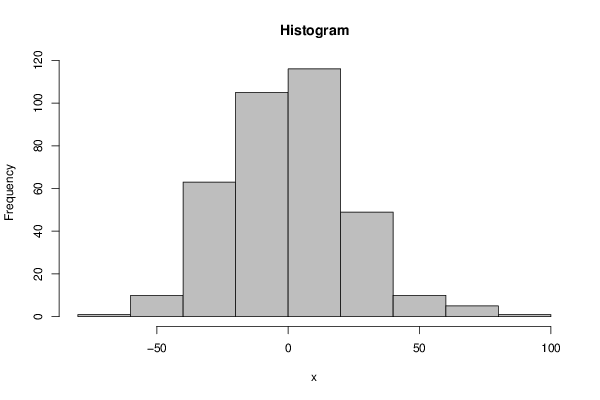
| Title produced by software | Histogram | ||||||||||||||||||||||||||||||||||||||||||||||||||||||||||||||||||||||||||||||||||||||||||||||||||||||||||||||||||||||||||||||||||||||||||||||||||||||||
| Date of computation | Sat, 10 Nov 2012 04:19:15 -0500 | ||||||||||||||||||||||||||||||||||||||||||||||||||||||||||||||||||||||||||||||||||||||||||||||||||||||||||||||||||||||||||||||||||||||||||||||||||||||||
| Cite this page as follows | Statistical Computations at FreeStatistics.org, Office for Research Development and Education, URL https://freestatistics.org/blog/index.php?v=date/2012/Nov/10/t1352539178cindnwc5uvkyrd4.htm/, Retrieved Thu, 11 Jun 2026 00:10:03 +0000 | ||||||||||||||||||||||||||||||||||||||||||||||||||||||||||||||||||||||||||||||||||||||||||||||||||||||||||||||||||||||||||||||||||||||||||||||||||||||||
| Statistical Computations at FreeStatistics.org, Office for Research Development and Education, URL https://freestatistics.org/blog/index.php?pk=187264, Retrieved Thu, 11 Jun 2026 00:10:03 +0000 | |||||||||||||||||||||||||||||||||||||||||||||||||||||||||||||||||||||||||||||||||||||||||||||||||||||||||||||||||||||||||||||||||||||||||||||||||||||||||
| QR Codes: | |||||||||||||||||||||||||||||||||||||||||||||||||||||||||||||||||||||||||||||||||||||||||||||||||||||||||||||||||||||||||||||||||||||||||||||||||||||||||
|
| |||||||||||||||||||||||||||||||||||||||||||||||||||||||||||||||||||||||||||||||||||||||||||||||||||||||||||||||||||||||||||||||||||||||||||||||||||||||||
| Original text written by user: | |||||||||||||||||||||||||||||||||||||||||||||||||||||||||||||||||||||||||||||||||||||||||||||||||||||||||||||||||||||||||||||||||||||||||||||||||||||||||
| IsPrivate? | No (this computation is public) | ||||||||||||||||||||||||||||||||||||||||||||||||||||||||||||||||||||||||||||||||||||||||||||||||||||||||||||||||||||||||||||||||||||||||||||||||||||||||
| User-defined keywords | |||||||||||||||||||||||||||||||||||||||||||||||||||||||||||||||||||||||||||||||||||||||||||||||||||||||||||||||||||||||||||||||||||||||||||||||||||||||||
| Estimated Impact | 467 | ||||||||||||||||||||||||||||||||||||||||||||||||||||||||||||||||||||||||||||||||||||||||||||||||||||||||||||||||||||||||||||||||||||||||||||||||||||||||
Tree of Dependent Computations | |||||||||||||||||||||||||||||||||||||||||||||||||||||||||||||||||||||||||||||||||||||||||||||||||||||||||||||||||||||||||||||||||||||||||||||||||||||||||
| Family? (F = Feedback message, R = changed R code, M = changed R Module, P = changed Parameters, D = changed Data) | |||||||||||||||||||||||||||||||||||||||||||||||||||||||||||||||||||||||||||||||||||||||||||||||||||||||||||||||||||||||||||||||||||||||||||||||||||||||||
| - [Univariate Data Series] [data set] [2008-12-01 19:54:57] [b98453cac15ba1066b407e146608df68] - RMPD [Histogram] [Histogram TA Movi...] [2012-11-10 09:19:15] [64435dfec13c3cda39d1733fd4b6eb52] [Current] | |||||||||||||||||||||||||||||||||||||||||||||||||||||||||||||||||||||||||||||||||||||||||||||||||||||||||||||||||||||||||||||||||||||||||||||||||||||||||
| Feedback Forum | |||||||||||||||||||||||||||||||||||||||||||||||||||||||||||||||||||||||||||||||||||||||||||||||||||||||||||||||||||||||||||||||||||||||||||||||||||||||||
Post a new message | |||||||||||||||||||||||||||||||||||||||||||||||||||||||||||||||||||||||||||||||||||||||||||||||||||||||||||||||||||||||||||||||||||||||||||||||||||||||||
Dataset | |||||||||||||||||||||||||||||||||||||||||||||||||||||||||||||||||||||||||||||||||||||||||||||||||||||||||||||||||||||||||||||||||||||||||||||||||||||||||
| Dataseries X: | |||||||||||||||||||||||||||||||||||||||||||||||||||||||||||||||||||||||||||||||||||||||||||||||||||||||||||||||||||||||||||||||||||||||||||||||||||||||||
NA NA NA NA NA NA -6.14157407407407 2.76675925925926 -2.47476851851854 -24.749212962963 -27.3419907407408 -24.0996296296296 -33.0386574074074 -8.16893518518521 -7.48046296296292 7.31495370370374 37.2350925925925 -3.20490740740735 51.4375925925926 27.5334259259259 4.37939814814808 30.0091203703704 -13.662824074074 -0.0871296296296009 28.6988425925926 45.4268981481482 31.4987037037038 19.1482870370371 12.1559259259259 -21.496574074074 -5.81240740740742 -26.7249074074074 -3.03726851851854 -15.2283796296296 6.97884259259257 23.2045370370371 -14.9094907407408 -25.0981018518518 -17.2137962962962 -11.4850462962962 -4.57740740740738 -37.1465740740741 -13.4457407407407 -5.92074074074074 22.5502314814815 26.9341203703704 29.5996759259259 9.35870370370372 -17.2886574074074 -17.2439351851852 -27.3471296296296 -1.68921296296298 16.6309259259259 -28.5215740740741 3.86675925925925 20.9292592592593 22.5293981481481 14.5757870370371 5.99134259259262 2.15870370370371 -9.53865740740738 -30.7189351851852 -18.6679629629629 15.4607870370371 11.4434259259259 -46.9799074074074 -33.029074074074 -35.5249074074074 -24.1331018518519 -30.8908796296296 -25.2169907407408 -8.68712962962957 21.4780092592593 39.6810648148148 52.869537037037 61.0149537037037 52.9142592592593 -24.8965740740741 -2.71657407407406 9.32925925925923 28.7460648148148 0.100787037037037 4.27467592592592 -0.216296296296264 0.0946759259259693 -9.41060185185182 -4.65129629629627 29.5566203703704 8.38509259259257 -40.0507407407407 -33.4207407407407 -9.84990740740739 -8.51226851851851 4.63412037037045 9.95384259259265 13.6003703703704 -15.642824074074 -21.7314351851851 2.63203703703704 5.66495370370376 36.0350925925926 0.678425925925978 5.86675925925925 -14.7165740740741 -14.6414351851852 -15.536712962963 14.9830092592592 20.7587037037037 2.93634259259267 -16.4564351851852 -20.4554629629629 -2.01421296296292 15.955925925926 -12.2924074074073 -23.616574074074 -37.3499074074074 -39.5247685185184 -47.3783796296295 -21.7961574074074 -20.3746296296297 1.50300925925922 41.0018981481482 53.2570370370371 72.7816203703704 62.4142592592594 22.8575925925927 31.9167592592593 15.3375925925926 -15.9414351851852 -21.074212962963 -26.3378240740741 13.0378703703704 13.0613425925926 18.8977314814815 11.2487037037037 -16.5350462962962 -15.9232407407407 -40.571574074074 -27.9457407407407 -16.3624074074074 -9.31226851851858 10.463287037037 29.2288425925926 14.6670370370371 -1.53865740740736 -35.1522685185184 14.1362037037037 -2.88087962962953 -7.30657407407398 -6.28824074074072 -18.5915740740741 -16.6540740740741 -50.5581018518519 -23.1158796296297 -12.1378240740741 26.8212037037036 30.8696759259259 47.6102314814815 41.982037037037 24.4857870370371 22.5642592592593 15.8117592592592 10.8917592592592 -1.67490740740749 -14.4956018518519 -6.92421296296294 -13.1711574074073 3.17537037037044 -2.75949074074066 -17.1856018518518 -4.57629629629628 -5.08504629629624 28.2600925925926 -15.821574074074 -28.1582407407407 3.16675925925927 -19.3414351851851 -26.6575462962963 0.703842592592707 1.51287037037042 12.3113425925926 28.0435648148148 9.04870370370378 3.87745370370374 19.1892592592593 6.17425925925932 -9.37074074074064 -14.041574074074 -21.6247685185184 -11.8242129629629 15.6955092592593 9.66287037037034 11.8113425925926 1.26439814814819 2.88620370370376 5.62745370370379 -0.677407407407372 22.8034259259259 -25.4957407407407 -2.61657407407404 -9.81226851851858 3.21328703703711 -3.37532407407406 7.47537037037034 -9.85949074074063 8.23939814814821 -12.1971296296295 11.3482870370372 8.30592592592598 24.1367592592593 -7.65407407407406 4.95009259259257 -1.65810185185188 6.99245370370375 8.51217592592593 0.99620370370377 -23.0969907407408 -41.2189351851852 -26.7679629629629 -9.88087962962965 19.6517592592592 28.503425925926 0.687592592592637 9.50009259259258 -4.15393518518511 8.29245370370376 0.0538425925926163 8.6920370370371 -16.0969907407407 -22.5647685185185 -24.1971296296297 -16.4017129629629 -19.4524074074073 23.1200925925927 10.8625925925926 11.758425925926 25.0418981481482 47.388287037037 22.5413425925926 3.72953703703706 -33.892824074074 -19.3856018518518 -29.7721296296296 -30.0725462962963 -24.6399074074074 36.2325925925927 24.0375925925926 13.5542592592593 17.6377314814815 24.3049537037037 9.39967592592598 -6.65379629629626 -33.080324074074 -36.1772685185185 -32.1429629629629 -15.0225462962962 -20.2274074074074 14.4950925925926 16.1292592592592 10.758425925926 30.1293981481481 25.8341203703704 -17.200324074074 -36.5537962962963 -42.7261574074074 -22.7189351851852 -16.4971296296296 -5.61004629629616 -15.2982407407408 24.0784259259259 16.958425925926 4.39592592592589 17.0293981481481 18.7841203703704 23.3080092592593 17.3712037037038 15.1238425925926 3.36856481481487 -5.6137962962963 -16.8350462962963 -28.0690740740741 7.57009259259257 16.7042592592592 21.4625925925926 17.6293981481481 6.27162037037033 9.65800925925925 -3.07462962962961 -0.1636574074073 -9.79393518518503 -4.38046296296289 -14.5475462962963 -26.2149074074074 13.8367592592594 19.6834259259259 25.333425925926 29.0335648148148 31.163287037037 -6.09615740740742 -17.620462962963 -29.9219907407407 -15.2564351851852 -20.292962962963 -8.63504629629631 -21.3857407407407 11.6825925925927 6.35425925925927 1.20842592592595 12.9752314814815 -12.9450462962962 -6.92115740740735 -11.5871296296296 5.02384259259264 4.81023148148148 -17.3262962962963 -31.9267129629629 -38.8232407407407 -3.39240740740735 -11.6249074074072 -43.8749074074073 -22.0872685185184 -51.7450462962962 -38.1128240740741 -25.0037962962963 83.6113425925927 64.8768981481481 72.0028703703705 39.7274537037038 25.3475925925926 36.1200925925926 21.1250925925926 2.67092592592621 8.20439814814836 3.57578703703712 -9.66282407407391 -5.1662962962962 25.9655092592593 8.42273148148149 -15.2471296296296 -34.5100462962963 -69.9024074074075 -6.36324074074071 13.4334259259261 20.6459259259261 8.90856481481501 6.64245370370372 13.512175925926 6.48370370370378 19.3655092592594 42.8352314814816 15.8487037037039 -37.4892129629629 -52.5899074074074 12.6409259259258 -4.3207407407408 18.6209259259259 15.1252314814816 17.5007870370372 15.249675925926 -24.970462962963 10.3113425925927 -7.58560185185195 -3.97212962962965 -36.776712962963 -32.7899074074074 -15.1049074074074 NA NA NA NA NA NA | |||||||||||||||||||||||||||||||||||||||||||||||||||||||||||||||||||||||||||||||||||||||||||||||||||||||||||||||||||||||||||||||||||||||||||||||||||||||||
Tables (Output of Computation) | |||||||||||||||||||||||||||||||||||||||||||||||||||||||||||||||||||||||||||||||||||||||||||||||||||||||||||||||||||||||||||||||||||||||||||||||||||||||||
| |||||||||||||||||||||||||||||||||||||||||||||||||||||||||||||||||||||||||||||||||||||||||||||||||||||||||||||||||||||||||||||||||||||||||||||||||||||||||
Figures (Output of Computation) | |||||||||||||||||||||||||||||||||||||||||||||||||||||||||||||||||||||||||||||||||||||||||||||||||||||||||||||||||||||||||||||||||||||||||||||||||||||||||
Input Parameters & R Code | |||||||||||||||||||||||||||||||||||||||||||||||||||||||||||||||||||||||||||||||||||||||||||||||||||||||||||||||||||||||||||||||||||||||||||||||||||||||||
| Parameters (Session): | |||||||||||||||||||||||||||||||||||||||||||||||||||||||||||||||||||||||||||||||||||||||||||||||||||||||||||||||||||||||||||||||||||||||||||||||||||||||||
| par2 = grey ; par3 = FALSE ; par4 = Unknown ; | |||||||||||||||||||||||||||||||||||||||||||||||||||||||||||||||||||||||||||||||||||||||||||||||||||||||||||||||||||||||||||||||||||||||||||||||||||||||||
| Parameters (R input): | |||||||||||||||||||||||||||||||||||||||||||||||||||||||||||||||||||||||||||||||||||||||||||||||||||||||||||||||||||||||||||||||||||||||||||||||||||||||||
| par1 = ; par2 = grey ; par3 = FALSE ; par4 = Unknown ; | |||||||||||||||||||||||||||||||||||||||||||||||||||||||||||||||||||||||||||||||||||||||||||||||||||||||||||||||||||||||||||||||||||||||||||||||||||||||||
| R code (references can be found in the software module): | |||||||||||||||||||||||||||||||||||||||||||||||||||||||||||||||||||||||||||||||||||||||||||||||||||||||||||||||||||||||||||||||||||||||||||||||||||||||||
par1 <- as.numeric(par1) | |||||||||||||||||||||||||||||||||||||||||||||||||||||||||||||||||||||||||||||||||||||||||||||||||||||||||||||||||||||||||||||||||||||||||||||||||||||||||