Free Statistics
of Irreproducible Research!
Description of Statistical Computation | |||||||||||||||||||||||||||||||||||||||||||||||||||||||||||||||||||||||||||||||||
|---|---|---|---|---|---|---|---|---|---|---|---|---|---|---|---|---|---|---|---|---|---|---|---|---|---|---|---|---|---|---|---|---|---|---|---|---|---|---|---|---|---|---|---|---|---|---|---|---|---|---|---|---|---|---|---|---|---|---|---|---|---|---|---|---|---|---|---|---|---|---|---|---|---|---|---|---|---|---|---|---|---|
| Author's title | Bootstrap Plot (gemiddelde consumptieprijzen aardappelen/kg, 2006-2011), 50... | ||||||||||||||||||||||||||||||||||||||||||||||||||||||||||||||||||||||||||||||||
| Author | *Unverified author* | ||||||||||||||||||||||||||||||||||||||||||||||||||||||||||||||||||||||||||||||||
| R Software Module | rwasp_bootstrapplot.wasp | ||||||||||||||||||||||||||||||||||||||||||||||||||||||||||||||||||||||||||||||||
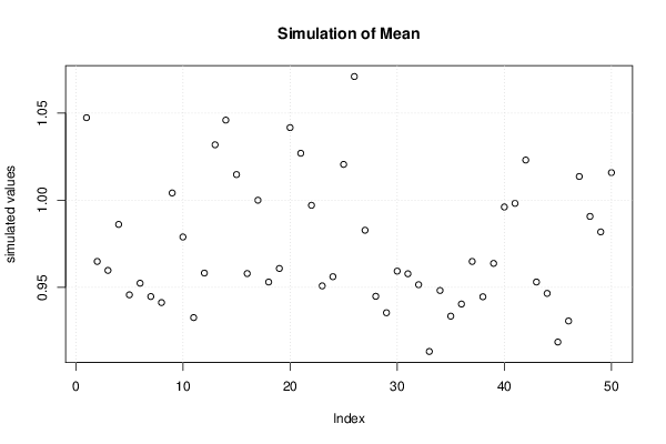
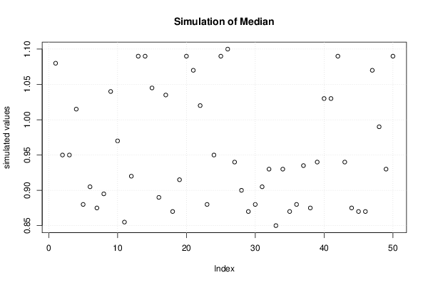
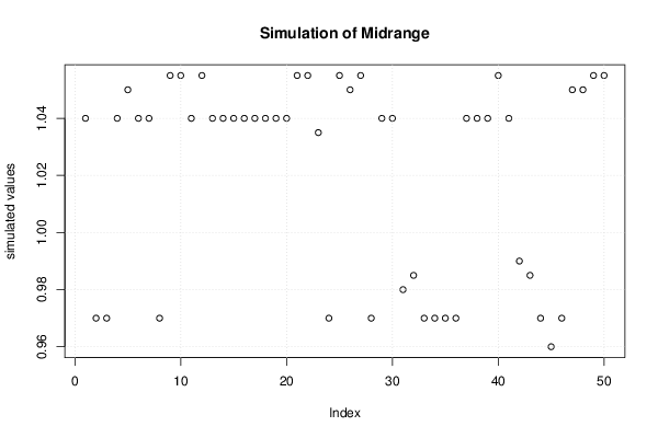
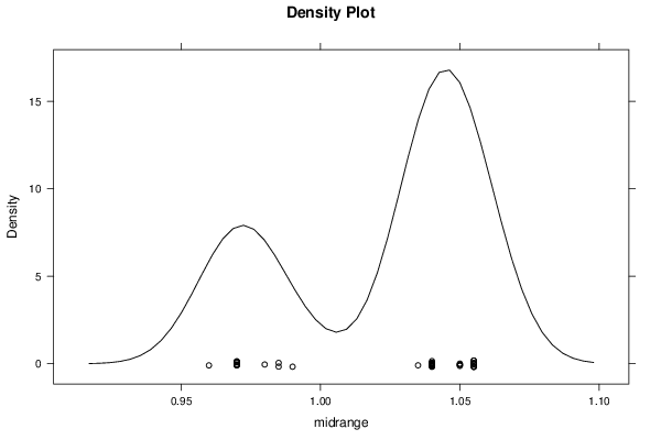
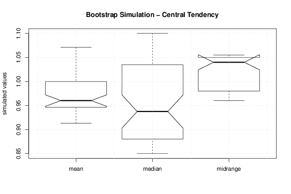
| Title produced by software | Blocked Bootstrap Plot - Central Tendency | ||||||||||||||||||||||||||||||||||||||||||||||||||||||||||||||||||||||||||||||||
| Date of computation | Thu, 27 Dec 2012 15:38:33 -0500 | ||||||||||||||||||||||||||||||||||||||||||||||||||||||||||||||||||||||||||||||||
| Cite this page as follows | Statistical Computations at FreeStatistics.org, Office for Research Development and Education, URL https://freestatistics.org/blog/index.php?v=date/2012/Dec/27/t1356640782j2rtr2ny1x75pme.htm/, Retrieved Sat, 05 Jul 2025 09:46:00 +0000 | ||||||||||||||||||||||||||||||||||||||||||||||||||||||||||||||||||||||||||||||||
| Statistical Computations at FreeStatistics.org, Office for Research Development and Education, URL https://freestatistics.org/blog/index.php?pk=204788, Retrieved Sat, 05 Jul 2025 09:46:00 +0000 | |||||||||||||||||||||||||||||||||||||||||||||||||||||||||||||||||||||||||||||||||
| QR Codes: | |||||||||||||||||||||||||||||||||||||||||||||||||||||||||||||||||||||||||||||||||
|
| |||||||||||||||||||||||||||||||||||||||||||||||||||||||||||||||||||||||||||||||||
| Original text written by user: | |||||||||||||||||||||||||||||||||||||||||||||||||||||||||||||||||||||||||||||||||
| IsPrivate? | No (this computation is public) | ||||||||||||||||||||||||||||||||||||||||||||||||||||||||||||||||||||||||||||||||
| User-defined keywords | |||||||||||||||||||||||||||||||||||||||||||||||||||||||||||||||||||||||||||||||||
| Estimated Impact | 245 | ||||||||||||||||||||||||||||||||||||||||||||||||||||||||||||||||||||||||||||||||
Tree of Dependent Computations | |||||||||||||||||||||||||||||||||||||||||||||||||||||||||||||||||||||||||||||||||
| Family? (F = Feedback message, R = changed R code, M = changed R Module, P = changed Parameters, D = changed Data) | |||||||||||||||||||||||||||||||||||||||||||||||||||||||||||||||||||||||||||||||||
| - [(Partial) Autocorrelation Function] [Autocorrelatie In...] [2012-11-12 10:59:56] [41982c7b3984978a38ca838fef047984] - RMPD [Bootstrap Plot - Central Tendency] [Bootstrap Plot (m...] [2012-12-27 20:12:14] [41982c7b3984978a38ca838fef047984] - R P [Bootstrap Plot - Central Tendency] [Bootstrap Plot (m...] [2012-12-27 20:14:03] [41982c7b3984978a38ca838fef047984] - RMPD [Blocked Bootstrap Plot - Central Tendency] [Bootstrap Plot (g...] [2012-12-27 20:38:33] [97ff841fcf87514e420f2e9629cfd808] [Current] - R D [Blocked Bootstrap Plot - Central Tendency] [Bootstrap Plot (g...] [2012-12-27 20:42:04] [41982c7b3984978a38ca838fef047984] - [Blocked Bootstrap Plot - Central Tendency] [Bootstrap Plot (g...] [2012-12-27 20:44:01] [41982c7b3984978a38ca838fef047984] - RM D [Variability] [Spreidingsmaten S...] [2012-12-27 20:59:10] [41982c7b3984978a38ca838fef047984] - RM D [Standard Deviation Plot] [Spreidingsgrafiek...] [2012-12-27 21:03:45] [41982c7b3984978a38ca838fef047984] - RM D [Standard Deviation-Mean Plot] [Spreidings- en ge...] [2012-12-27 21:11:16] [41982c7b3984978a38ca838fef047984] - RM D [Variability] [Spreidingsmaten g...] [2012-12-27 21:17:49] [41982c7b3984978a38ca838fef047984] - RM [Standard Deviation Plot] [Spreidingsgrafiek...] [2012-12-27 21:20:17] [41982c7b3984978a38ca838fef047984] - RM [Standard Deviation-Mean Plot] [Spreidings- en ge...] [2012-12-27 21:24:21] [41982c7b3984978a38ca838fef047984] - RM D [Classical Decomposition] [Decompositie Insc...] [2012-12-27 21:30:41] [41982c7b3984978a38ca838fef047984] | |||||||||||||||||||||||||||||||||||||||||||||||||||||||||||||||||||||||||||||||||
| Feedback Forum | |||||||||||||||||||||||||||||||||||||||||||||||||||||||||||||||||||||||||||||||||
Post a new message | |||||||||||||||||||||||||||||||||||||||||||||||||||||||||||||||||||||||||||||||||
Dataset | |||||||||||||||||||||||||||||||||||||||||||||||||||||||||||||||||||||||||||||||||
| Dataseries X: | |||||||||||||||||||||||||||||||||||||||||||||||||||||||||||||||||||||||||||||||||
0,75 0,75 0,77 0,78 0,79 1,01 1,16 1,14 1,12 1,1 1,1 1,1 1,1 1,09 1,09 1,1 1,1 1,17 1,15 1,04 0,94 0,88 0,85 0,85 0,85 0,84 0,83 0,8 0,78 1,02 1,19 1,1 0,96 0,87 0,83 0,82 0,81 0,78 0,79 0,8 0,79 0,97 1,01 0,92 0,87 0,84 0,81 0,81 0,83 0,83 0,85 0,88 0,89 1,21 1,32 1,33 1,23 1,16 1,12 1,06 1,08 1,09 1,03 1,04 1,05 1,19 1,14 1,05 0,95 0,87 0,86 0,85 | |||||||||||||||||||||||||||||||||||||||||||||||||||||||||||||||||||||||||||||||||
Tables (Output of Computation) | |||||||||||||||||||||||||||||||||||||||||||||||||||||||||||||||||||||||||||||||||
| |||||||||||||||||||||||||||||||||||||||||||||||||||||||||||||||||||||||||||||||||
Figures (Output of Computation) | |||||||||||||||||||||||||||||||||||||||||||||||||||||||||||||||||||||||||||||||||
Input Parameters & R Code | |||||||||||||||||||||||||||||||||||||||||||||||||||||||||||||||||||||||||||||||||
| Parameters (Session): | |||||||||||||||||||||||||||||||||||||||||||||||||||||||||||||||||||||||||||||||||
| par1 = 50 ; par2 = 12 ; | |||||||||||||||||||||||||||||||||||||||||||||||||||||||||||||||||||||||||||||||||
| Parameters (R input): | |||||||||||||||||||||||||||||||||||||||||||||||||||||||||||||||||||||||||||||||||
| par1 = 50 ; par2 = 12 ; | |||||||||||||||||||||||||||||||||||||||||||||||||||||||||||||||||||||||||||||||||
| R code (references can be found in the software module): | |||||||||||||||||||||||||||||||||||||||||||||||||||||||||||||||||||||||||||||||||
par1 <- as.numeric(par1) | |||||||||||||||||||||||||||||||||||||||||||||||||||||||||||||||||||||||||||||||||