Free Statistics
of Irreproducible Research!
Description of Statistical Computation | ||||||||||||||||||||||||||||||||||||||||||||||||||||||||||||||||||||||||||||||||||||||||||||||||||||||||||||||
|---|---|---|---|---|---|---|---|---|---|---|---|---|---|---|---|---|---|---|---|---|---|---|---|---|---|---|---|---|---|---|---|---|---|---|---|---|---|---|---|---|---|---|---|---|---|---|---|---|---|---|---|---|---|---|---|---|---|---|---|---|---|---|---|---|---|---|---|---|---|---|---|---|---|---|---|---|---|---|---|---|---|---|---|---|---|---|---|---|---|---|---|---|---|---|---|---|---|---|---|---|---|---|---|---|---|---|---|---|---|---|
| Author's title | Granger Causality Test (Effective reproduction Rate (Rt) and Daily Changes ... | |||||||||||||||||||||||||||||||||||||||||||||||||||||||||||||||||||||||||||||||||||||||||||||||||||||||||||||
| Author | *Unverified author* | |||||||||||||||||||||||||||||||||||||||||||||||||||||||||||||||||||||||||||||||||||||||||||||||||||||||||||||
| R Software Module | rwasp_grangercausality.wasp | |||||||||||||||||||||||||||||||||||||||||||||||||||||||||||||||||||||||||||||||||||||||||||||||||||||||||||||
| Title produced by software | Bivariate Granger Causality | |||||||||||||||||||||||||||||||||||||||||||||||||||||||||||||||||||||||||||||||||||||||||||||||||||||||||||||
| Date of computation | Mon, 02 Nov 2020 14:35:00 +0100 | |||||||||||||||||||||||||||||||||||||||||||||||||||||||||||||||||||||||||||||||||||||||||||||||||||||||||||||
| Cite this page as follows | Statistical Computations at FreeStatistics.org, Office for Research Development and Education, URL https://freestatistics.org/blog/index.php?v=date/2020/Nov/02/t16043257103rgpy4em30x1b68.htm/, Retrieved Sun, 19 Apr 2026 23:20:18 +0000 | |||||||||||||||||||||||||||||||||||||||||||||||||||||||||||||||||||||||||||||||||||||||||||||||||||||||||||||
| Statistical Computations at FreeStatistics.org, Office for Research Development and Education, URL https://freestatistics.org/blog/index.php?pk=319286, Retrieved Sun, 19 Apr 2026 23:20:18 +0000 | ||||||||||||||||||||||||||||||||||||||||||||||||||||||||||||||||||||||||||||||||||||||||||||||||||||||||||||||
| QR Codes: | ||||||||||||||||||||||||||||||||||||||||||||||||||||||||||||||||||||||||||||||||||||||||||||||||||||||||||||||
|
| ||||||||||||||||||||||||||||||||||||||||||||||||||||||||||||||||||||||||||||||||||||||||||||||||||||||||||||||
| Original text written by user: | The effective reproduction number (Rt) characterizes the COVID-19 spread rate, defined as the average number of secondary infectious cases produced by a primary infectious case. It's used to define the potential for spread at a specific time. If Rt > 1, the virus will spread out and the disease will become an epidemic; if Rt = 1, the virus will spread locally and the disease is endemic; if Rt < 1, the virus will stop spreading and the disease will disappear eventually. | |||||||||||||||||||||||||||||||||||||||||||||||||||||||||||||||||||||||||||||||||||||||||||||||||||||||||||||
| IsPrivate? | No (this computation is public) | |||||||||||||||||||||||||||||||||||||||||||||||||||||||||||||||||||||||||||||||||||||||||||||||||||||||||||||
| User-defined keywords | COVID-19, Granger Causality, coronavirus, causation | |||||||||||||||||||||||||||||||||||||||||||||||||||||||||||||||||||||||||||||||||||||||||||||||||||||||||||||
| Estimated Impact | 590 | |||||||||||||||||||||||||||||||||||||||||||||||||||||||||||||||||||||||||||||||||||||||||||||||||||||||||||||
Tree of Dependent Computations | ||||||||||||||||||||||||||||||||||||||||||||||||||||||||||||||||||||||||||||||||||||||||||||||||||||||||||||||
| Family? (F = Feedback message, R = changed R code, M = changed R Module, P = changed Parameters, D = changed Data) | ||||||||||||||||||||||||||||||||||||||||||||||||||||||||||||||||||||||||||||||||||||||||||||||||||||||||||||||
| - [Bivariate Granger Causality] [Granger Causality...] [2020-11-02 13:35:00] [d41d8cd98f00b204e9800998ecf8427e] [Current] | ||||||||||||||||||||||||||||||||||||||||||||||||||||||||||||||||||||||||||||||||||||||||||||||||||||||||||||||
| Feedback Forum | ||||||||||||||||||||||||||||||||||||||||||||||||||||||||||||||||||||||||||||||||||||||||||||||||||||||||||||||
Post a new message | ||||||||||||||||||||||||||||||||||||||||||||||||||||||||||||||||||||||||||||||||||||||||||||||||||||||||||||||
Dataset | ||||||||||||||||||||||||||||||||||||||||||||||||||||||||||||||||||||||||||||||||||||||||||||||||||||||||||||||
| Dataseries X: | ||||||||||||||||||||||||||||||||||||||||||||||||||||||||||||||||||||||||||||||||||||||||||||||||||||||||||||||
3.13268334113438 3.23680175944288 2.88201788002659 2.84782400562102 2.71810149609755 2.44065988251605 2.23863300087288 2.19514358951984 2.07242710819333 1.97638531045049 1.8236525166409 1.72029114049977 1.70546130097739 1.65189829656141 1.58557088082452 1.53894154228052 1.49890695043382 1.43296771300372 1.37572106858207 1.31423896028701 1.27620068211179 1.23719073110979 1.19271666481855 1.13273494034869 1.10008117322411 1.06044449130108 1.03677437952325 1.02239801876862 1.00505120394206 1.00228622950044 0.996280565089463 0.991838295278499 1.00731273460677 0.994311104170129 0.991710369994506 1.0033423688786 1.00696376428079 1.02490805403557 1.02701356651755 0.99542207468205 0.989034234689879 0.985004268905044 0.969155426103344 0.978515180807519 0.964710637720008 0.958262701191528 0.96779905761605 0.973896659619999 0.965037828796574 0.962528307649591 0.931864319745562 0.928295648674492 0.912508443218754 0.907232210922053 0.914672848097462 0.907180332185469 0.920934890065206 0.926441998360512 0.93379692152295 0.941178044132804 0.967004251523819 0.962413397673273 0.983596585704783 0.97641511760466 0.968251869809063 0.956481286638731 0.976924780768252 0.958734424114706 0.956082934690587 0.933412009280572 0.928026320506047 0.947944321990947 0.975753943365337 0.973851641940048 0.971206612381403 0.988559795454045 1.00000716273254 0.991154837705696 0.997439579256495 0.984444459756276 0.977552760781905 0.983153216023638 0.966344206791663 0.978198607446143 0.993148066564895 0.992304739349162 1.01673010010048 1.02436458134856 1.03486638638068 1.06400087170071 1.08440752216375 1.09834323737949 1.11799150592697 1.13583550166198 1.14658171273992 1.17628421610042 1.20537865074223 1.20475666592013 1.22204768277372 1.24161241025079 1.23357487859282 1.23952191204384 1.22886276385055 1.21937613097321 1.23750440412637 1.23952983100443 1.21029425558432 1.1739173894269 1.17227938102655 1.14893115937397 1.16214641209852 1.15272007173472 1.14426130206149 1.15843072361637 1.16605354979179 1.15428275707241 1.16036415630809 1.14358083358139 1.13374779242332 1.14062940178436 1.12139015721312 1.10150220246048 1.08636184599063 1.07513620858528 1.05493059592553 1.05282553633104 1.0250868838384 1.02297926010526 1.02813978914988 1.00932479770758 0.995826213799495 1.00051752098514 1.0014652334907 0.998755287241208 0.986161601577111 0.970138474598601 0.959655141801341 0.941806761941038 0.934331200923467 0.906914443528443 0.90500092463194 0.902386780589967 0.915024819499958 0.927914125485945 0.953211578757473 0.934911815023185 0.954023952851286 0.943176562431584 0.968967316713541 0.953422452935177 0.948387360630864 0.921140580418662 0.931012875548141 0.918096781913661 0.910584453847272 0.880492915267113 0.892675641160665 0.892150684081569 0.916914204819174 0.910119824087103 0.918106572010934 0.938504776903768 0.94292251946294 0.957639200494041 0.968032599722392 0.962076403731244 0.982489196564965 0.970671992408838 0.968404822516469 0.987432873894959 0.983369171615036 0.971386059732191 0.940899820213446 0.897349008498947 0.891553872879251 0.885427050387315 0.896898456954474 0.90455205325297 0.935131024647991 0.985379980765945 1.0357580497798 1.04584663162617 1.06560420943611 1.05507324918537 1.05317158472571 1.04747823838632 1.10469357834037 1.08248738128835 1.06247193897359 1.04746683064293 1.0446198617158 1.03904768090427 1.03219190851599 0.961937290742673 0.979425771696781 0.996538467352552 0.999946765189486 1.01328936614376 1.02839631206512 1.01920753474297 1.03558329907384 1.02816505016485 1.05145171522686 1.07903197304015 1.07148241431483 1.06994350548963 1.08407024940122 1.07315126230609 1.08932340936452 1.09863711849644 1.09927176679916 1.11168977921657 1.09612294570503 1.08518071711069 1.11323983150607 1.11113647331645 1.09519919396093 1.0955607901256 1.11272620180715 1.15363536166823 1.15017795006617 1.13526166644376 1.13544017437059 1.14075946110941 1.146400928383 1.14693019704503 | ||||||||||||||||||||||||||||||||||||||||||||||||||||||||||||||||||||||||||||||||||||||||||||||||||||||||||||||
| Dataseries Y: | ||||||||||||||||||||||||||||||||||||||||||||||||||||||||||||||||||||||||||||||||||||||||||||||||||||||||||||||
13.6402425130708 19.325194499493 18.1960956532842 26.731111662798 34.0550781033943 32.1034368181463 36.525740632464 54.3090474602526 56.5763507885267 59.4810486267574 57.4595974666094 66.8019798554015 80.0324687549287 78.3661373931851 92.2370560146211 97.1176768337172 100.155923997844 85.5474488720292 91.6209079883297 95.2995848743648 97.1753458608085 105.167058930883 101.788868028113 89.1077524919295 81.8262790186637 78.2811514585242 86.7797449246119 91.0806402608427 95.6789863683866 99.5731633030261 84.533688080003 77.9472781437851 86.2667941046945 79.0308488107112 88.9226045628469 101.470170773135 101.879924386678 96.522775291091 82.2542439039202 70.3349665677322 74.8908197079457 84.51547680829 89.5539286488991 103.8649530034 84.9920050847813 74.3687632521717 71.0300301047801 74.5539111812543 76.326474961324 84.3515753628726 81.5925676983462 75.786207233837 57.2319565701963 59.0318372578356 69.0692831836756 63.639289001236 82.9007440497333 76.7756863302458 72.8997206673194 54.9950053614439 66.8201911271145 63.8365777781273 71.3547977836627 77.8987147525503 71.1392977350584 64.3404229621882 61.0502532060314 55.6020477518788 59.265548578153 56.424590190918 69.652043878493 73.9134814593456 72.3715937876411 58.2001891829399 52.7034203375524 64.8746202657709 60.6374643805357 65.9824726283144 76.3932496242719 66.2829586115797 53.9903502052743 53.201195097709 55.762913985344 63.2113241159794 70.4381637741061 75.488756462524 76.6846299716806 58.813301997279 60.4765981470705 72.2289388258889 78.6393064688808 85.5686953556944 95.0780144018561 97.9037967293303 79.2463488593156 92.5345067859341 108.651482251979 104.59036865997 123.096055932376 137.56491130839 128.565507870194 119.447731165863 123.499739122015 140.14787667969 155.779218233387 167.303918015793 159.536810630179 138.854876388064 151.708999005522 135.522213664577 182.604421466703 179.629913753572 192.059106697725 205.538482977331 182.616562314512 178.777019195011 180.537442127272 203.28939092077 205.265313901635 234.858630435333 218.599000007536 190.499007754308 186.03421097266 188.204387518464 195.604234257865 216.480422064919 209.702793775714 221.925592307119 201.786961004444 166.478340364801 171.771750009393 199.780685904057 216.492562912728 205.848074596453 203.823588224353 175.76001851455 143.66568733226 136.120150419155 174.451842163163 162.86036771781 181.053428159142 177.095511773507 169.061305736102 139.999151294034 151.0503580119 142.390898312347 173.040468605402 157.812810241344 196.062551262643 143.950997255765 125.700267787341 109.082482349188 137.686319786477 143.686933815926 133.804283699646 146.367025969695 134.808938855816 104.496277089453 114.904018873458 116.042223355523 136.86681255939 139.258559577703 140.260179521921 139.704735734673 107.331165052783 104.75730531734 129.099705173776 123.178006655085 133.264015972159 152.103576559305 133.834635819168 94.5407818863213 73.0393404171194 81.152461965281 101.852607479109 110.357271369101 144.266659298791 124.610626696511 105.312749104587 103.057586624122 118.986378949132 117.034737663884 135.795382740273 147.887667157735 133.770896368173 109.983940298984 159.242395070818 118.345949227223 116.694793925241 134.007642900442 153.5635135083 136.220312413577 110.548489722088 101.130227034491 127.840092213624 125.709373423198 135.88947431079 165.531354235723 151.954851173648 107.649862307762 120.05780876825 127.336247029563 152.792569672448 170.666932858802 174.354715380693 165.850051490701 135.431157306012 126.486387682955 159.196866891536 180.704378784642 193.209452027599 209.930434672127 174.667342211767 146.367025969695 177.241201947211 183.190217373472 190.538465509686 217.627732182841 254.189895358731 254.138296755544 184.562133175855 202.746087981331 223.488726462489 237.833138148464 268.67999721841 301.460286301891 | ||||||||||||||||||||||||||||||||||||||||||||||||||||||||||||||||||||||||||||||||||||||||||||||||||||||||||||||
Tables (Output of Computation) | ||||||||||||||||||||||||||||||||||||||||||||||||||||||||||||||||||||||||||||||||||||||||||||||||||||||||||||||
| ||||||||||||||||||||||||||||||||||||||||||||||||||||||||||||||||||||||||||||||||||||||||||||||||||||||||||||||
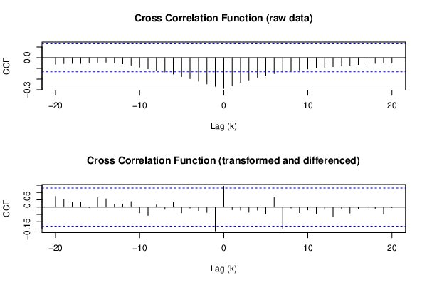
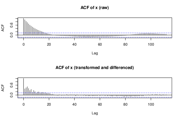
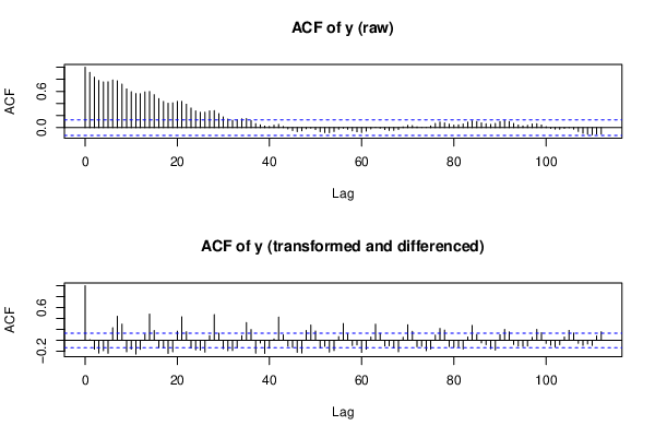
Figures (Output of Computation) | ||||||||||||||||||||||||||||||||||||||||||||||||||||||||||||||||||||||||||||||||||||||||||||||||||||||||||||||
Input Parameters & R Code | ||||||||||||||||||||||||||||||||||||||||||||||||||||||||||||||||||||||||||||||||||||||||||||||||||||||||||||||
| Parameters (Session): | ||||||||||||||||||||||||||||||||||||||||||||||||||||||||||||||||||||||||||||||||||||||||||||||||||||||||||||||
| par1 = 1 ; par2 = 1 ; par3 = 0 ; par4 = 1 ; par5 = 1 ; par6 = 1 ; par7 = 0 ; par8 = 1 ; | ||||||||||||||||||||||||||||||||||||||||||||||||||||||||||||||||||||||||||||||||||||||||||||||||||||||||||||||
| Parameters (R input): | ||||||||||||||||||||||||||||||||||||||||||||||||||||||||||||||||||||||||||||||||||||||||||||||||||||||||||||||
| par1 = 1 ; par2 = 1 ; par3 = 0 ; par4 = 1 ; par5 = 1 ; par6 = 1 ; par7 = 0 ; par8 = 1 ; | ||||||||||||||||||||||||||||||||||||||||||||||||||||||||||||||||||||||||||||||||||||||||||||||||||||||||||||||
| R code (references can be found in the software module): | ||||||||||||||||||||||||||||||||||||||||||||||||||||||||||||||||||||||||||||||||||||||||||||||||||||||||||||||
par8 <- '1' | ||||||||||||||||||||||||||||||||||||||||||||||||||||||||||||||||||||||||||||||||||||||||||||||||||||||||||||||