Free Statistics
of Irreproducible Research!
Description of Statistical Computation | |||||||||||||||||||||||||||||||||||||||||||||||||||||||||||||
|---|---|---|---|---|---|---|---|---|---|---|---|---|---|---|---|---|---|---|---|---|---|---|---|---|---|---|---|---|---|---|---|---|---|---|---|---|---|---|---|---|---|---|---|---|---|---|---|---|---|---|---|---|---|---|---|---|---|---|---|---|---|
| Author's title | |||||||||||||||||||||||||||||||||||||||||||||||||||||||||||||
| Author | *Unverified author* | ||||||||||||||||||||||||||||||||||||||||||||||||||||||||||||
| R Software Module | rwasp_linear_regression.wasp | ||||||||||||||||||||||||||||||||||||||||||||||||||||||||||||
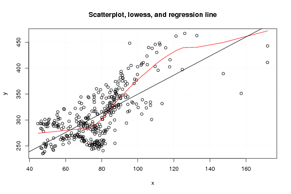
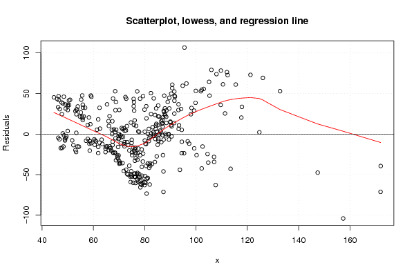
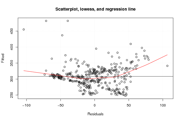
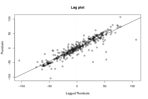
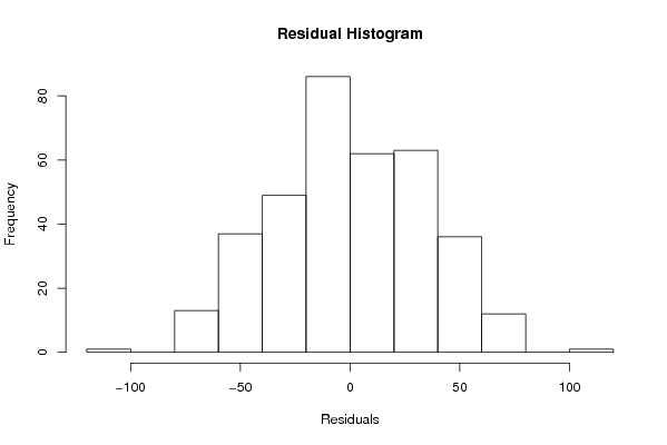
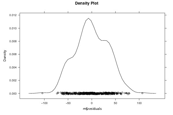
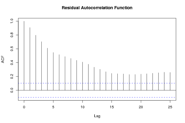
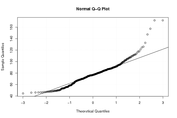
| Title produced by software | Linear Regression Graphical Model Validation | ||||||||||||||||||||||||||||||||||||||||||||||||||||||||||||
| Date of computation | Tue, 26 Feb 2008 03:22:06 -0700 | ||||||||||||||||||||||||||||||||||||||||||||||||||||||||||||
| Cite this page as follows | Statistical Computations at FreeStatistics.org, Office for Research Development and Education, URL https://freestatistics.org/blog/index.php?v=date/2008/Feb/26/t12040214435my4uqfrs09mgrk.htm/, Retrieved Wed, 13 May 2026 15:00:41 +0000 | ||||||||||||||||||||||||||||||||||||||||||||||||||||||||||||
| Statistical Computations at FreeStatistics.org, Office for Research Development and Education, URL https://freestatistics.org/blog/index.php?pk=9091, Retrieved Wed, 13 May 2026 15:00:41 +0000 | |||||||||||||||||||||||||||||||||||||||||||||||||||||||||||||
| QR Codes: | |||||||||||||||||||||||||||||||||||||||||||||||||||||||||||||
|
| |||||||||||||||||||||||||||||||||||||||||||||||||||||||||||||
| Original text written by user: | |||||||||||||||||||||||||||||||||||||||||||||||||||||||||||||
| IsPrivate? | No (this computation is public) | ||||||||||||||||||||||||||||||||||||||||||||||||||||||||||||
| User-defined keywords | |||||||||||||||||||||||||||||||||||||||||||||||||||||||||||||
| Estimated Impact | 2774 | ||||||||||||||||||||||||||||||||||||||||||||||||||||||||||||
Tree of Dependent Computations | |||||||||||||||||||||||||||||||||||||||||||||||||||||||||||||
| Family? (F = Feedback message, R = changed R code, M = changed R Module, P = changed Parameters, D = changed Data) | |||||||||||||||||||||||||||||||||||||||||||||||||||||||||||||
| - [Linear Regression Graphical Model Validation] [Colombia Coffee -...] [2008-02-26 10:22:06] [d41d8cd98f00b204e9800998ecf8427e] [Current] - PD [Linear Regression Graphical Model Validation] [Linear Regression...] [2008-12-22 14:50:39] [33f4701c7363e8b81858dafbf0350eed] - D [Linear Regression Graphical Model Validation] [Linear Regression...] [2008-12-22 20:24:18] [b187fac1a1b0cb3920f54366df47fea3] - [Linear Regression Graphical Model Validation] [linear regression...] [2008-12-22 20:49:59] [b641c14ac36cb6fee377f3b099dcac19] - M D [Linear Regression Graphical Model Validation] [WS6: Toturial ass...] [2010-11-05 10:55:30] [1fd136673b2a4fecb5c545b9b4a05d64] - P [Linear Regression Graphical Model Validation] [ws6.3 tutorial] [2010-11-15 08:23:24] [e4076051fbfb461c886b1e223cd7862f] - D [Linear Regression Graphical Model Validation] [Workshop 6_Tutorial] [2011-11-15 11:03:26] [f722e8e78b9e5c5ebaa2263f273aa636] - RM [Linear Regression Graphical Model Validation] [linear regression] [2011-11-15 14:55:12] [d31984dff2665bea309b726bae3d5241] - RM [Linear Regression Graphical Model Validation] [] [2011-11-15 22:01:41] [74be16979710d4c4e7c6647856088456] - M D [Linear Regression Graphical Model Validation] [Scatterplot Tutorial] [2010-11-05 11:55:49] [aeb27d5c05332f2e597ad139ee63fbe4] - D [Linear Regression Graphical Model Validation] [Simple Linear Reg...] [2010-11-12 11:48:01] [aeb27d5c05332f2e597ad139ee63fbe4] - D [Linear Regression Graphical Model Validation] [Simple Linear Reg...] [2010-12-17 13:47:08] [aeb27d5c05332f2e597ad139ee63fbe4] - RMPD [Multiple Regression] [WS6: Toturial ass...] [2010-11-05 12:08:30] [1fd136673b2a4fecb5c545b9b4a05d64] - P [Multiple Regression] [ws6.4 tutorial] [2010-11-15 08:32:05] [e4076051fbfb461c886b1e223cd7862f] - P [Multiple Regression] [Ws 6 Tutorial Ass...] [2011-11-13 21:56:59] [74be16979710d4c4e7c6647856088456] - R P [Multiple Regression] [Ws 6 Tutorial Ass...] [2011-11-13 22:00:46] [74be16979710d4c4e7c6647856088456] - RM [Multiple Regression] [regression] [2011-11-15 15:06:25] [d31984dff2665bea309b726bae3d5241] - RM [Multiple Regression] [] [2011-11-15 22:07:29] [74be16979710d4c4e7c6647856088456] - RM D [Linear Regression Graphical Model Validation] [Regression Model 1] [2010-11-05 17:43:27] [97ad38b1c3b35a5feca8b85f7bc7b3ff] - P [Linear Regression Graphical Model Validation] [Vraag 3: Lineair ...] [2010-11-11 10:18:38] [39c51da0be01189e8a44eb69e891b7a1] - RM [Linear Regression Graphical Model Validation] [WS 6 - 11] [2011-11-15 14:55:02] [74be16979710d4c4e7c6647856088456] - RM D [Linear Regression Graphical Model Validation] [Regressiemodel 1] [2010-11-06 16:54:19] [97ad38b1c3b35a5feca8b85f7bc7b3ff] - PD [Linear Regression Graphical Model Validation] [Regressiemodel 1] [2010-11-20 19:37:29] [97ad38b1c3b35a5feca8b85f7bc7b3ff] - PD [Linear Regression Graphical Model Validation] [Regressiemodel 1] [2010-11-20 19:54:37] [97ad38b1c3b35a5feca8b85f7bc7b3ff] - RMPD [Univariate Data Series] [Bestedingen] [2010-12-10 12:35:43] [97ad38b1c3b35a5feca8b85f7bc7b3ff] - RMPD [Mean Plot] [Mean plot Schiphol] [2010-12-10 12:51:13] [97ad38b1c3b35a5feca8b85f7bc7b3ff] - D [Linear Regression Graphical Model Validation] [Regressiemodel 1] [2010-12-10 12:24:47] [97ad38b1c3b35a5feca8b85f7bc7b3ff] - RMPD [Spectral Analysis] [Spectral Analysis...] [2010-12-10 14:16:07] [97ad38b1c3b35a5feca8b85f7bc7b3ff] - R [Spectral Analysis] [Paper - Spectral ...] [2011-12-20 14:36:26] [69d59b79aaf660457acc70a0ef0bfdab] - RMPD [(Partial) Autocorrelation Function] [Autocorrelatiefun...] [2010-12-10 14:34:45] [97ad38b1c3b35a5feca8b85f7bc7b3ff] - R P [(Partial) Autocorrelation Function] [Paper - autocorre...] [2011-12-20 15:27:59] [69d59b79aaf660457acc70a0ef0bfdab] - RMPD [Multiple Regression] [Schiphol: MR - Mo...] [2010-12-10 14:47:34] [97ad38b1c3b35a5feca8b85f7bc7b3ff] - R D [Linear Regression Graphical Model Validation] [] [2011-11-15 17:48:12] [06c08141d7d783218a8164fd2ea166f2] - [Linear Regression Graphical Model Validation] [] [2011-12-18 15:51:24] [06c08141d7d783218a8164fd2ea166f2] - R P [Linear Regression Graphical Model Validation] [] [2011-11-15 21:43:38] [ec2187f7727da5d5d939740b21b8b68a] - R PD [Linear Regression Graphical Model Validation] [] [2011-12-19 15:58:44] [ec2187f7727da5d5d939740b21b8b68a] - R [Linear Regression Graphical Model Validation] [Paper - Hypothese...] [2011-12-19 16:27:20] [69d59b79aaf660457acc70a0ef0bfdab] F RMPD [Chi-Squared and McNemar Tests] [WS6 - Chi kwadraa...] [2010-11-07 14:08:40] [8ef49741e164ec6343c90c7935194465] - R [Chi-Squared and McNemar Tests] [Workshop 6, Chi-S...] [2010-11-09 11:02:54] [8ffb4cfa64b4677df0d2c448735a40bb] - P [Chi-Squared and McNemar Tests] [Workshop 6, Chi-S...] [2010-11-09 16:29:28] [8ffb4cfa64b4677df0d2c448735a40bb] - P [Chi-Squared and McNemar Tests] [Workshop 6, Chi-S...] [2010-11-09 16:32:35] [8ffb4cfa64b4677df0d2c448735a40bb] - P [Chi-Squared and McNemar Tests] [Workshop 6, Chi-S...] [2010-11-09 16:41:58] [8ffb4cfa64b4677df0d2c448735a40bb] F [Chi-Squared and McNemar Tests] [WS6 Hap-Con] [2010-11-11 17:20:45] [afe9379cca749d06b3d6872e02cc47ed] - [Chi-Squared and McNemar Tests] [] [2010-11-15 17:01:17] [b64b273f7a25c5bb07ff2f026b8ce952] - R D [Chi-Squared Test, McNemar Test, and Fisher Exact Test] [ws 6 - 1.3] [2011-11-14 20:51:16] [4b648d52023f19d55c572f0eddd72b1f] - R PD [Chi-Squared Test, McNemar Test, and Fisher Exact Test] [ws 6 - 1.2] [2011-11-14 20:52:27] [4b648d52023f19d55c572f0eddd72b1f] - R PD [Chi-Squared Test, McNemar Test, and Fisher Exact Test] [ws 6 - 1.1] [2011-11-14 20:53:08] [4b648d52023f19d55c572f0eddd72b1f] - R PD [Chi-Squared Test, McNemar Test, and Fisher Exact Test] [ws 6 - 1.4] [2011-11-14 20:54:13] [4b648d52023f19d55c572f0eddd72b1f] - R PD [Chi-Squared Test, McNemar Test, and Fisher Exact Test] [ws 6 - 1.5] [2011-11-14 20:55:43] [4b648d52023f19d55c572f0eddd72b1f] [Truncated] | |||||||||||||||||||||||||||||||||||||||||||||||||||||||||||||
| Feedback Forum | |||||||||||||||||||||||||||||||||||||||||||||||||||||||||||||
Post a new message | |||||||||||||||||||||||||||||||||||||||||||||||||||||||||||||
Dataset | |||||||||||||||||||||||||||||||||||||||||||||||||||||||||||||
| Dataseries X: | |||||||||||||||||||||||||||||||||||||||||||||||||||||||||||||
87.28 87.28 87.09 86.92 87.59 90.72 90.69 90.3 89.55 88.94 88.41 87.82 87.07 86.82 86.4 86.02 85.66 85.32 85 84.67 83.94 82.83 81.95 81.19 80.48 78.86 69.47 68.77 70.06 73.95 75.8 77.79 81.57 83.07 84.34 85.1 85.25 84.26 83.63 86.44 85.3 84.1 83.36 82.48 81.58 80.47 79.34 82.13 81.69 80.7 79.88 79.16 78.38 77.42 76.47 75.46 74.48 78.27 80.7 79.91 78.75 77.78 81.14 81.08 80.03 78.91 78.01 76.9 75.97 81.93 80.27 78.67 77.42 76.16 74.7 76.39 76.04 74.65 73.29 71.79 74.39 74.91 74.54 73.08 72.75 71.32 70.38 70.35 70.01 69.36 67.77 69.26 69.8 68.38 67.62 68.39 66.95 65.21 66.64 63.45 60.66 62.34 60.32 58.64 60.46 58.59 61.87 61.85 67.44 77.06 91.74 93.15 94.15 93.11 91.51 89.96 88.16 86.98 88.03 86.24 84.65 83.23 81.7 80.25 78.8 77.51 76.2 75.04 74 75.49 77.14 76.15 76.27 78.19 76.49 77.31 76.65 74.99 73.51 72.07 70.59 71.96 76.29 74.86 74.93 71.9 71.01 77.47 75.78 76.6 76.07 74.57 73.02 72.65 73.16 71.53 69.78 67.98 69.96 72.16 70.47 68.86 67.37 65.87 72.16 71.34 69.93 68.44 67.16 66.01 67.25 70.91 69.75 68.59 67.48 66.31 64.81 66.58 65.97 64.7 64.7 60.94 59.08 58.42 57.77 57.11 53.31 49.96 49.4 48.84 48.3 47.74 47.24 46.76 46.29 48.9 49.23 48.53 48.03 54.34 53.79 53.24 52.96 52.17 51.7 58.55 78.2 77.03 76.19 77.15 75.87 95.47 109.67 112.28 112.01 107.93 105.96 105.06 102.98 102.2 105.23 101.85 99.89 96.23 94.76 91.51 91.63 91.54 85.23 87.83 87.38 84.44 85.19 84.03 86.73 102.52 104.45 106.98 107.02 99.26 94.45 113.44 157.33 147.38 171.89 171.95 132.71 126.02 121.18 115.45 110.48 117.85 117.63 124.65 109.59 111.27 99.78 98.21 99.2 97.97 89.55 87.91 93.34 94.42 93.2 90.29 91.46 89.98 88.35 88.41 82.44 79.89 75.69 75.66 84.5 96.73 87.48 82.39 83.48 79.31 78.16 72.77 72.45 68.46 67.62 68.76 70.07 68.55 65.3 58.96 59.17 62.37 66.28 55.62 55.23 55.85 56.75 50.89 53.88 52.95 55.08 53.61 58.78 61.85 55.91 53.32 46.41 44.57 50 50 53.36 46.23 50.45 49.07 45.85 48.45 49.96 46.53 50.51 47.58 48.05 46.84 47.67 49.16 55.54 55.82 58.22 56.19 57.77 63.19 54.76 55.74 62.54 61.39 69.6 79.23 80 93.68 107.63 100.18 97.3 90.45 80.64 80.58 75.82 85.59 89.35 89.42 104.73 95.32 89.27 90.44 86.97 79.98 81.22 87.35 83.64 82.22 94.4 102.18 | |||||||||||||||||||||||||||||||||||||||||||||||||||||||||||||
| Dataseries Y: | |||||||||||||||||||||||||||||||||||||||||||||||||||||||||||||
255 280.2 299.9 339.2 374.2 393.5 389.2 381.7 375.2 369 357.4 352.1 346.5 342.9 340.3 328.3 322.9 314.3 308.9 294 285.6 281.2 280.3 278.8 274.5 270.4 263.4 259.9 258 262.7 284.7 311.3 322.1 327 331.3 333.3 321.4 327 320 314.7 316.7 314.4 321.3 318.2 307.2 301.3 287.5 277.7 274.4 258.8 253.3 251 248.4 249.5 246.1 244.5 243.6 244 240.8 249.8 248 259.4 260.5 260.8 261.3 259.5 256.6 257.9 256.5 254.2 253.3 253.8 255.5 257.1 257.3 253.2 252.8 252 250.7 252.2 250 251 253.4 251.2 255.6 261.1 258.9 259.9 261.2 264.7 267.1 266.4 267.7 268.6 267.5 268.5 268.5 270.5 270.9 270.1 269.3 269.8 270.1 264.9 263.7 264.8 263.7 255.9 276.2 360.1 380.5 373.7 369.8 366.6 359.3 345.8 326.2 324.5 328.1 327.5 324.4 316.5 310.9 301.5 291.7 290.4 287.4 277.7 281.6 288 276 272.9 283 283.3 276.8 284.5 282.7 281.2 287.4 283.1 284 285.5 289.2 292.5 296.4 305.2 303.9 311.5 316.3 316.7 322.5 317.1 309.8 303.8 290.3 293.7 291.7 296.5 289.1 288.5 293.8 297.7 305.4 302.7 302.5 303 294.5 294.1 294.5 297.1 289.4 292.4 287.9 286.6 280.5 272.4 269.2 270.6 267.3 262.5 266.8 268.8 263.1 261.2 266 262.5 265.2 261.3 253.7 249.2 239.1 236.4 235.2 245.2 246.2 247.7 251.4 253.3 254.8 250 249.3 241.5 243.3 248 253 252.9 251.5 251.6 253.5 259.8 334.1 448 445.8 445 448.2 438.2 439.8 423.4 410.8 408.4 406.7 405.9 402.7 405.1 399.6 386.5 381.4 375.2 357.7 359 355 352.7 344.4 343.8 338 339 333.3 334.4 328.3 330.7 330 331.6 351.2 389.4 410.9 442.8 462.8 466.9 461.7 439.2 430.3 416.1 402.5 397.3 403.3 395.9 387.8 378.6 377.1 370.4 362 350.3 348.2 344.6 343.5 342.8 347.6 346.6 349.5 342.1 342 342.8 339.3 348.2 333.7 334.7 354 367.7 363.3 358.4 353.1 343.1 344.6 344.4 333.9 331.7 324.3 321.2 322.4 321.7 320.5 312.8 309.7 315.6 309.7 304.6 302.5 301.5 298.8 291.3 293.6 294.6 285.9 297.6 301.1 293.8 297.7 292.9 292.1 287.2 288.2 283.8 299.9 292.4 293.3 300.8 293.7 293.1 294.4 292.1 291.9 282.5 277.9 287.5 289.2 285.6 293.2 290.8 283.1 275 287.8 287.8 287.4 284 277.8 277.6 304.9 294 300.9 324 332.9 341.6 333.4 348.2 344.7 344.7 329.3 323.5 323.2 317.4 330.1 329.2 334.9 315.8 315.4 319.6 317.3 313.8 315.8 311.3 | |||||||||||||||||||||||||||||||||||||||||||||||||||||||||||||
Tables (Output of Computation) | |||||||||||||||||||||||||||||||||||||||||||||||||||||||||||||
| |||||||||||||||||||||||||||||||||||||||||||||||||||||||||||||
Figures (Output of Computation) | |||||||||||||||||||||||||||||||||||||||||||||||||||||||||||||
Input Parameters & R Code | |||||||||||||||||||||||||||||||||||||||||||||||||||||||||||||
| Parameters (Session): | |||||||||||||||||||||||||||||||||||||||||||||||||||||||||||||
| par1 = 0 ; | |||||||||||||||||||||||||||||||||||||||||||||||||||||||||||||
| Parameters (R input): | |||||||||||||||||||||||||||||||||||||||||||||||||||||||||||||
| par1 = 0 ; | |||||||||||||||||||||||||||||||||||||||||||||||||||||||||||||
| R code (references can be found in the software module): | |||||||||||||||||||||||||||||||||||||||||||||||||||||||||||||
par1 <- as.numeric(par1) | |||||||||||||||||||||||||||||||||||||||||||||||||||||||||||||