Repository of Reproducible Computations

Free Statistics

of Irreproducible Research!

Author's title

Author

*Unverified author*

R Software Module

rwasp_autocorrelation.wasp

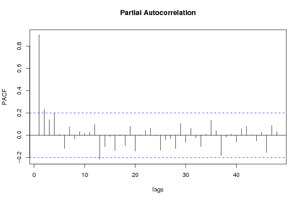
Title produced by software

(Partial) Autocorrelation Function

Date of computation

Sat, 06 Dec 2008 07:57:34 -0700

Cite this page as follows

Statistical Computations at FreeStatistics.org, Office for Research Development and Education, URL https://freestatistics.org/blog/index.php?v=date/2008/Dec/06/t1228575574ezbsmogz8psni34.htm/, Retrieved Sat, 18 May 2024 05:32:32 +0000

Statistical Computations at FreeStatistics.org, Office for Research Development and Education, URL https://freestatistics.org/blog/index.php?pk=29681, Retrieved Sat, 18 May 2024 05:32:32 +0000

QR Codes:

Paste this QR Code to cite your computation.

Original text written by user:

IsPrivate?

No (this computation is public)

User-defined keywords

Estimated Impact

162

Family? (F = Feedback message, R = changed R code, M = changed R Module, P = changed Parameters, D = changed Data)

-     [Mean Plot] [Opgave 6-1/2- Ins...] [2008-12-04 18:02:51] [ad379bf1a8c2f692a4d6e13d12ca6606]
- RMPD    [(Partial) Autocorrelation Function] [Opgave 6bis - 2/1...] [2008-12-06 14:57:34] [c3b8efbffd908bee7ef47d968749a3e1] [Current]

Feedback Forum

Post a new message

Dataseries X:

Download CSV

Histogram

Boxplots

Summary of computational transaction
Raw Input	view raw input (R code)
Raw Output	view raw output of R engine
Computing time	1 seconds
R Server	'Gwilym Jenkins' @ 72.249.127.135

\begin{tabular}{lllllllll}
\hline
Summary of computational transaction \tabularnewline
Raw Input & view raw input (R code)  \tabularnewline
Raw Output & view raw output of R engine  \tabularnewline
Computing time & 1 seconds \tabularnewline
R Server & 'Gwilym Jenkins' @ 72.249.127.135 \tabularnewline
\hline
\end{tabular}
%Source: https://freestatistics.org/blog/index.php?pk=29681&T=0

[TABLE]
[ROW][C]Summary of computational transaction[/C][/ROW]
[ROW][C]Raw Input[/C][C]view raw input (R code) [/C][/ROW]
[ROW][C]Raw Output[/C][C]view raw output of R engine [/C][/ROW]
[ROW][C]Computing time[/C][C]1 seconds[/C][/ROW]
[ROW][C]R Server[/C][C]'Gwilym Jenkins' @ 72.249.127.135[/C][/ROW]
[/TABLE]
Source: https://freestatistics.org/blog/index.php?pk=29681&T=0

Globally Unique Identifier (entire table): ba.freestatistics.org/blog/index.php?pk=29681&T=0

As an alternative you can also use a QR Code:

The GUIDs for individual cells are displayed in the table below:

Summary of computational transaction
Raw Input	view raw input (R code)
Raw Output	view raw output of R engine
Computing time	1 seconds
R Server	'Gwilym Jenkins' @ 72.249.127.135

Autocorrelation Function
Time lag k	ACF(k)	T-STAT	P-value
1	0.903419	8.8517	0
2	0.858858	8.4151	0
3	0.829797	8.1303	0
4	0.825251	8.0858	0
5	0.801002	7.8482	0
6	0.755893	7.4062	0
7	0.737931	7.2302	0
8	0.712627	6.9823	0
9	0.697754	6.8366	0
10	0.673918	6.603	0
11	0.656911	6.4364	0
12	0.654822	6.4159	0
13	0.6062	5.9395	0
14	0.566678	5.5523	0
15	0.536312	5.2548	0
16	0.501309	4.9118	2e-06
17	0.471773	4.6224	6e-06
18	0.41853	4.1007	4.3e-05
19	0.40238	3.9425	7.7e-05
20	0.352204	3.4509	0.000416
21	0.323822	3.1728	0.001014
22	0.296609	2.9062	0.002271
23	0.283099	2.7738	0.003329
24	0.265743	2.6037	0.005343
25	0.208807	2.0459	0.021752
26	0.172217	1.6874	0.047389
27	0.140418	1.3758	0.086041
28	0.102428	1.0036	0.159051
29	0.078343	0.7676	0.222304
30	0.029757	0.2916	0.385628
31	0.015194	0.1489	0.440984
32	-0.022001	-0.2156	0.414894
33	-0.058662	-0.5748	0.283396
34	-0.083344	-0.8166	0.208088
35	-0.08425	-0.8255	0.205574
36	-0.08245	-0.8078	0.210589
37	-0.145063	-1.4213	0.079233
38	-0.172272	-1.6879	0.047337
39	-0.193122	-1.8922	0.030739
40	-0.209156	-2.0493	0.02158
41	-0.226378	-2.218	0.014455
42	-0.250251	-2.4519	0.008008
43	-0.25913	-2.5389	0.006363
44	-0.282744	-2.7703	0.003362
45	-0.292351	-2.8644	0.002566
46	-0.31695	-3.1055	0.001249
47	-0.312364	-3.0605	0.001433
48	-0.303536	-2.974	0.001858

\begin{tabular}{lllllllll}
\hline
Autocorrelation Function \tabularnewline
Time lag k & ACF(k) & T-STAT & P-value \tabularnewline
1 & 0.903419 & 8.8517 & 0 \tabularnewline
2 & 0.858858 & 8.4151 & 0 \tabularnewline
3 & 0.829797 & 8.1303 & 0 \tabularnewline
4 & 0.825251 & 8.0858 & 0 \tabularnewline
5 & 0.801002 & 7.8482 & 0 \tabularnewline
6 & 0.755893 & 7.4062 & 0 \tabularnewline
7 & 0.737931 & 7.2302 & 0 \tabularnewline
8 & 0.712627 & 6.9823 & 0 \tabularnewline
9 & 0.697754 & 6.8366 & 0 \tabularnewline
10 & 0.673918 & 6.603 & 0 \tabularnewline
11 & 0.656911 & 6.4364 & 0 \tabularnewline
12 & 0.654822 & 6.4159 & 0 \tabularnewline
13 & 0.6062 & 5.9395 & 0 \tabularnewline
14 & 0.566678 & 5.5523 & 0 \tabularnewline
15 & 0.536312 & 5.2548 & 0 \tabularnewline
16 & 0.501309 & 4.9118 & 2e-06 \tabularnewline
17 & 0.471773 & 4.6224 & 6e-06 \tabularnewline
18 & 0.41853 & 4.1007 & 4.3e-05 \tabularnewline
19 & 0.40238 & 3.9425 & 7.7e-05 \tabularnewline
20 & 0.352204 & 3.4509 & 0.000416 \tabularnewline
21 & 0.323822 & 3.1728 & 0.001014 \tabularnewline
22 & 0.296609 & 2.9062 & 0.002271 \tabularnewline
23 & 0.283099 & 2.7738 & 0.003329 \tabularnewline
24 & 0.265743 & 2.6037 & 0.005343 \tabularnewline
25 & 0.208807 & 2.0459 & 0.021752 \tabularnewline
26 & 0.172217 & 1.6874 & 0.047389 \tabularnewline
27 & 0.140418 & 1.3758 & 0.086041 \tabularnewline
28 & 0.102428 & 1.0036 & 0.159051 \tabularnewline
29 & 0.078343 & 0.7676 & 0.222304 \tabularnewline
30 & 0.029757 & 0.2916 & 0.385628 \tabularnewline
31 & 0.015194 & 0.1489 & 0.440984 \tabularnewline
32 & -0.022001 & -0.2156 & 0.414894 \tabularnewline
33 & -0.058662 & -0.5748 & 0.283396 \tabularnewline
34 & -0.083344 & -0.8166 & 0.208088 \tabularnewline
35 & -0.08425 & -0.8255 & 0.205574 \tabularnewline
36 & -0.08245 & -0.8078 & 0.210589 \tabularnewline
37 & -0.145063 & -1.4213 & 0.079233 \tabularnewline
38 & -0.172272 & -1.6879 & 0.047337 \tabularnewline
39 & -0.193122 & -1.8922 & 0.030739 \tabularnewline
40 & -0.209156 & -2.0493 & 0.02158 \tabularnewline
41 & -0.226378 & -2.218 & 0.014455 \tabularnewline
42 & -0.250251 & -2.4519 & 0.008008 \tabularnewline
43 & -0.25913 & -2.5389 & 0.006363 \tabularnewline
44 & -0.282744 & -2.7703 & 0.003362 \tabularnewline
45 & -0.292351 & -2.8644 & 0.002566 \tabularnewline
46 & -0.31695 & -3.1055 & 0.001249 \tabularnewline
47 & -0.312364 & -3.0605 & 0.001433 \tabularnewline
48 & -0.303536 & -2.974 & 0.001858 \tabularnewline
\hline
\end{tabular}
%Source: https://freestatistics.org/blog/index.php?pk=29681&T=1

[TABLE]
[ROW][C]Autocorrelation Function[/C][/ROW]
[ROW][C]Time lag k[/C][C]ACF(k)[/C][C]T-STAT[/C][C]P-value[/C][/ROW]
[ROW][C]1[/C][C]0.903419[/C][C]8.8517[/C][C]0[/C][/ROW]
[ROW][C]2[/C][C]0.858858[/C][C]8.4151[/C][C]0[/C][/ROW]
[ROW][C]3[/C][C]0.829797[/C][C]8.1303[/C][C]0[/C][/ROW]
[ROW][C]4[/C][C]0.825251[/C][C]8.0858[/C][C]0[/C][/ROW]
[ROW][C]5[/C][C]0.801002[/C][C]7.8482[/C][C]0[/C][/ROW]
[ROW][C]6[/C][C]0.755893[/C][C]7.4062[/C][C]0[/C][/ROW]
[ROW][C]7[/C][C]0.737931[/C][C]7.2302[/C][C]0[/C][/ROW]
[ROW][C]8[/C][C]0.712627[/C][C]6.9823[/C][C]0[/C][/ROW]
[ROW][C]9[/C][C]0.697754[/C][C]6.8366[/C][C]0[/C][/ROW]
[ROW][C]10[/C][C]0.673918[/C][C]6.603[/C][C]0[/C][/ROW]
[ROW][C]11[/C][C]0.656911[/C][C]6.4364[/C][C]0[/C][/ROW]
[ROW][C]12[/C][C]0.654822[/C][C]6.4159[/C][C]0[/C][/ROW]
[ROW][C]13[/C][C]0.6062[/C][C]5.9395[/C][C]0[/C][/ROW]
[ROW][C]14[/C][C]0.566678[/C][C]5.5523[/C][C]0[/C][/ROW]
[ROW][C]15[/C][C]0.536312[/C][C]5.2548[/C][C]0[/C][/ROW]
[ROW][C]16[/C][C]0.501309[/C][C]4.9118[/C][C]2e-06[/C][/ROW]
[ROW][C]17[/C][C]0.471773[/C][C]4.6224[/C][C]6e-06[/C][/ROW]
[ROW][C]18[/C][C]0.41853[/C][C]4.1007[/C][C]4.3e-05[/C][/ROW]
[ROW][C]19[/C][C]0.40238[/C][C]3.9425[/C][C]7.7e-05[/C][/ROW]
[ROW][C]20[/C][C]0.352204[/C][C]3.4509[/C][C]0.000416[/C][/ROW]
[ROW][C]21[/C][C]0.323822[/C][C]3.1728[/C][C]0.001014[/C][/ROW]
[ROW][C]22[/C][C]0.296609[/C][C]2.9062[/C][C]0.002271[/C][/ROW]
[ROW][C]23[/C][C]0.283099[/C][C]2.7738[/C][C]0.003329[/C][/ROW]
[ROW][C]24[/C][C]0.265743[/C][C]2.6037[/C][C]0.005343[/C][/ROW]
[ROW][C]25[/C][C]0.208807[/C][C]2.0459[/C][C]0.021752[/C][/ROW]
[ROW][C]26[/C][C]0.172217[/C][C]1.6874[/C][C]0.047389[/C][/ROW]
[ROW][C]27[/C][C]0.140418[/C][C]1.3758[/C][C]0.086041[/C][/ROW]
[ROW][C]28[/C][C]0.102428[/C][C]1.0036[/C][C]0.159051[/C][/ROW]
[ROW][C]29[/C][C]0.078343[/C][C]0.7676[/C][C]0.222304[/C][/ROW]
[ROW][C]30[/C][C]0.029757[/C][C]0.2916[/C][C]0.385628[/C][/ROW]
[ROW][C]31[/C][C]0.015194[/C][C]0.1489[/C][C]0.440984[/C][/ROW]
[ROW][C]32[/C][C]-0.022001[/C][C]-0.2156[/C][C]0.414894[/C][/ROW]
[ROW][C]33[/C][C]-0.058662[/C][C]-0.5748[/C][C]0.283396[/C][/ROW]
[ROW][C]34[/C][C]-0.083344[/C][C]-0.8166[/C][C]0.208088[/C][/ROW]
[ROW][C]35[/C][C]-0.08425[/C][C]-0.8255[/C][C]0.205574[/C][/ROW]
[ROW][C]36[/C][C]-0.08245[/C][C]-0.8078[/C][C]0.210589[/C][/ROW]
[ROW][C]37[/C][C]-0.145063[/C][C]-1.4213[/C][C]0.079233[/C][/ROW]
[ROW][C]38[/C][C]-0.172272[/C][C]-1.6879[/C][C]0.047337[/C][/ROW]
[ROW][C]39[/C][C]-0.193122[/C][C]-1.8922[/C][C]0.030739[/C][/ROW]
[ROW][C]40[/C][C]-0.209156[/C][C]-2.0493[/C][C]0.02158[/C][/ROW]
[ROW][C]41[/C][C]-0.226378[/C][C]-2.218[/C][C]0.014455[/C][/ROW]
[ROW][C]42[/C][C]-0.250251[/C][C]-2.4519[/C][C]0.008008[/C][/ROW]
[ROW][C]43[/C][C]-0.25913[/C][C]-2.5389[/C][C]0.006363[/C][/ROW]
[ROW][C]44[/C][C]-0.282744[/C][C]-2.7703[/C][C]0.003362[/C][/ROW]
[ROW][C]45[/C][C]-0.292351[/C][C]-2.8644[/C][C]0.002566[/C][/ROW]
[ROW][C]46[/C][C]-0.31695[/C][C]-3.1055[/C][C]0.001249[/C][/ROW]
[ROW][C]47[/C][C]-0.312364[/C][C]-3.0605[/C][C]0.001433[/C][/ROW]
[ROW][C]48[/C][C]-0.303536[/C][C]-2.974[/C][C]0.001858[/C][/ROW]
[/TABLE]
Source: https://freestatistics.org/blog/index.php?pk=29681&T=1

Globally Unique Identifier (entire table): ba.freestatistics.org/blog/index.php?pk=29681&T=1

As an alternative you can also use a QR Code:

The GUIDs for individual cells are displayed in the table below:

Autocorrelation Function
Time lag k	ACF(k)	T-STAT	P-value
1	0.903419	8.8517	0
2	0.858858	8.4151	0
3	0.829797	8.1303	0
4	0.825251	8.0858	0
5	0.801002	7.8482	0
6	0.755893	7.4062	0
7	0.737931	7.2302	0
8	0.712627	6.9823	0
9	0.697754	6.8366	0
10	0.673918	6.603	0
11	0.656911	6.4364	0
12	0.654822	6.4159	0
13	0.6062	5.9395	0
14	0.566678	5.5523	0
15	0.536312	5.2548	0
16	0.501309	4.9118	2e-06
17	0.471773	4.6224	6e-06
18	0.41853	4.1007	4.3e-05
19	0.40238	3.9425	7.7e-05
20	0.352204	3.4509	0.000416
21	0.323822	3.1728	0.001014
22	0.296609	2.9062	0.002271
23	0.283099	2.7738	0.003329
24	0.265743	2.6037	0.005343
25	0.208807	2.0459	0.021752
26	0.172217	1.6874	0.047389
27	0.140418	1.3758	0.086041
28	0.102428	1.0036	0.159051
29	0.078343	0.7676	0.222304
30	0.029757	0.2916	0.385628
31	0.015194	0.1489	0.440984
32	-0.022001	-0.2156	0.414894
33	-0.058662	-0.5748	0.283396
34	-0.083344	-0.8166	0.208088
35	-0.08425	-0.8255	0.205574
36	-0.08245	-0.8078	0.210589
37	-0.145063	-1.4213	0.079233
38	-0.172272	-1.6879	0.047337
39	-0.193122	-1.8922	0.030739
40	-0.209156	-2.0493	0.02158
41	-0.226378	-2.218	0.014455
42	-0.250251	-2.4519	0.008008
43	-0.25913	-2.5389	0.006363
44	-0.282744	-2.7703	0.003362
45	-0.292351	-2.8644	0.002566
46	-0.31695	-3.1055	0.001249
47	-0.312364	-3.0605	0.001433
48	-0.303536	-2.974	0.001858

Partial Autocorrelation Function
Time lag k	PACF(k)	T-STAT	P-value
1	0.903419	8.8517	0
2	0.232235	2.2754	0.012552
3	0.139586	1.3677	0.087307
4	0.200456	1.9641	0.026208
5	0.008862	0.0868	0.465496
6	-0.119694	-1.1728	0.121897
7	0.074581	0.7307	0.23336
8	-0.034075	-0.3339	0.369603
9	0.031888	0.3124	0.377691
10	0.015535	0.1522	0.43967
11	0.025805	0.2528	0.400468
12	0.097343	0.9538	0.171299
13	-0.214816	-2.1048	0.018962
14	-0.103812	-1.0171	0.155821
15	-0.011714	-0.1148	0.454434
16	-0.138872	-1.3607	0.088403
17	0.007998	0.0784	0.468851
18	-0.094344	-0.9244	0.178803
19	0.080894	0.7926	0.214983
20	-0.144051	-1.4114	0.080679
21	-0.004464	-0.0437	0.482602
22	0.043686	0.428	0.334793
23	0.063143	0.6187	0.268798
24	-0.006835	-0.067	0.473374
25	-0.135674	-1.3293	0.093445
26	-0.044242	-0.4335	0.332817
27	-0.033382	-0.3271	0.37216
28	-0.12067	-1.1823	0.119999
29	0.105623	1.0349	0.15166
30	-0.064893	-0.6358	0.263204
31	0.062394	0.6113	0.271211
32	-0.025184	-0.2468	0.402813
33	-0.102808	-1.0073	0.15816
34	0.009914	0.0971	0.46141
35	0.134437	1.3172	0.095452
36	0.042008	0.4116	0.340778
37	-0.183477	-1.7977	0.037685
38	-0.018077	-0.1771	0.429895
39	0.008843	0.0866	0.465567
40	-0.061286	-0.6005	0.274801
41	0.058966	0.5777	0.282393
42	0.079488	0.7788	0.218999
43	0.001213	0.0119	0.495271
44	-0.053116	-0.5204	0.301983
45	0.028804	0.2822	0.389193
46	-0.156857	-1.5369	0.063806
47	0.088469	0.8668	0.194103
48	0.031891	0.3125	0.377681

\begin{tabular}{lllllllll}
\hline
Partial Autocorrelation Function \tabularnewline
Time lag k & PACF(k) & T-STAT & P-value \tabularnewline
1 & 0.903419 & 8.8517 & 0 \tabularnewline
2 & 0.232235 & 2.2754 & 0.012552 \tabularnewline
3 & 0.139586 & 1.3677 & 0.087307 \tabularnewline
4 & 0.200456 & 1.9641 & 0.026208 \tabularnewline
5 & 0.008862 & 0.0868 & 0.465496 \tabularnewline
6 & -0.119694 & -1.1728 & 0.121897 \tabularnewline
7 & 0.074581 & 0.7307 & 0.23336 \tabularnewline
8 & -0.034075 & -0.3339 & 0.369603 \tabularnewline
9 & 0.031888 & 0.3124 & 0.377691 \tabularnewline
10 & 0.015535 & 0.1522 & 0.43967 \tabularnewline
11 & 0.025805 & 0.2528 & 0.400468 \tabularnewline
12 & 0.097343 & 0.9538 & 0.171299 \tabularnewline
13 & -0.214816 & -2.1048 & 0.018962 \tabularnewline
14 & -0.103812 & -1.0171 & 0.155821 \tabularnewline
15 & -0.011714 & -0.1148 & 0.454434 \tabularnewline
16 & -0.138872 & -1.3607 & 0.088403 \tabularnewline
17 & 0.007998 & 0.0784 & 0.468851 \tabularnewline
18 & -0.094344 & -0.9244 & 0.178803 \tabularnewline
19 & 0.080894 & 0.7926 & 0.214983 \tabularnewline
20 & -0.144051 & -1.4114 & 0.080679 \tabularnewline
21 & -0.004464 & -0.0437 & 0.482602 \tabularnewline
22 & 0.043686 & 0.428 & 0.334793 \tabularnewline
23 & 0.063143 & 0.6187 & 0.268798 \tabularnewline
24 & -0.006835 & -0.067 & 0.473374 \tabularnewline
25 & -0.135674 & -1.3293 & 0.093445 \tabularnewline
26 & -0.044242 & -0.4335 & 0.332817 \tabularnewline
27 & -0.033382 & -0.3271 & 0.37216 \tabularnewline
28 & -0.12067 & -1.1823 & 0.119999 \tabularnewline
29 & 0.105623 & 1.0349 & 0.15166 \tabularnewline
30 & -0.064893 & -0.6358 & 0.263204 \tabularnewline
31 & 0.062394 & 0.6113 & 0.271211 \tabularnewline
32 & -0.025184 & -0.2468 & 0.402813 \tabularnewline
33 & -0.102808 & -1.0073 & 0.15816 \tabularnewline
34 & 0.009914 & 0.0971 & 0.46141 \tabularnewline
35 & 0.134437 & 1.3172 & 0.095452 \tabularnewline
36 & 0.042008 & 0.4116 & 0.340778 \tabularnewline
37 & -0.183477 & -1.7977 & 0.037685 \tabularnewline
38 & -0.018077 & -0.1771 & 0.429895 \tabularnewline
39 & 0.008843 & 0.0866 & 0.465567 \tabularnewline
40 & -0.061286 & -0.6005 & 0.274801 \tabularnewline
41 & 0.058966 & 0.5777 & 0.282393 \tabularnewline
42 & 0.079488 & 0.7788 & 0.218999 \tabularnewline
43 & 0.001213 & 0.0119 & 0.495271 \tabularnewline
44 & -0.053116 & -0.5204 & 0.301983 \tabularnewline
45 & 0.028804 & 0.2822 & 0.389193 \tabularnewline
46 & -0.156857 & -1.5369 & 0.063806 \tabularnewline
47 & 0.088469 & 0.8668 & 0.194103 \tabularnewline
48 & 0.031891 & 0.3125 & 0.377681 \tabularnewline
\hline
\end{tabular}
%Source: https://freestatistics.org/blog/index.php?pk=29681&T=2

[TABLE]
[ROW][C]Partial Autocorrelation Function[/C][/ROW]
[ROW][C]Time lag k[/C][C]PACF(k)[/C][C]T-STAT[/C][C]P-value[/C][/ROW]
[ROW][C]1[/C][C]0.903419[/C][C]8.8517[/C][C]0[/C][/ROW]
[ROW][C]2[/C][C]0.232235[/C][C]2.2754[/C][C]0.012552[/C][/ROW]
[ROW][C]3[/C][C]0.139586[/C][C]1.3677[/C][C]0.087307[/C][/ROW]
[ROW][C]4[/C][C]0.200456[/C][C]1.9641[/C][C]0.026208[/C][/ROW]
[ROW][C]5[/C][C]0.008862[/C][C]0.0868[/C][C]0.465496[/C][/ROW]
[ROW][C]6[/C][C]-0.119694[/C][C]-1.1728[/C][C]0.121897[/C][/ROW]
[ROW][C]7[/C][C]0.074581[/C][C]0.7307[/C][C]0.23336[/C][/ROW]
[ROW][C]8[/C][C]-0.034075[/C][C]-0.3339[/C][C]0.369603[/C][/ROW]
[ROW][C]9[/C][C]0.031888[/C][C]0.3124[/C][C]0.377691[/C][/ROW]
[ROW][C]10[/C][C]0.015535[/C][C]0.1522[/C][C]0.43967[/C][/ROW]
[ROW][C]11[/C][C]0.025805[/C][C]0.2528[/C][C]0.400468[/C][/ROW]
[ROW][C]12[/C][C]0.097343[/C][C]0.9538[/C][C]0.171299[/C][/ROW]
[ROW][C]13[/C][C]-0.214816[/C][C]-2.1048[/C][C]0.018962[/C][/ROW]
[ROW][C]14[/C][C]-0.103812[/C][C]-1.0171[/C][C]0.155821[/C][/ROW]
[ROW][C]15[/C][C]-0.011714[/C][C]-0.1148[/C][C]0.454434[/C][/ROW]
[ROW][C]16[/C][C]-0.138872[/C][C]-1.3607[/C][C]0.088403[/C][/ROW]
[ROW][C]17[/C][C]0.007998[/C][C]0.0784[/C][C]0.468851[/C][/ROW]
[ROW][C]18[/C][C]-0.094344[/C][C]-0.9244[/C][C]0.178803[/C][/ROW]
[ROW][C]19[/C][C]0.080894[/C][C]0.7926[/C][C]0.214983[/C][/ROW]
[ROW][C]20[/C][C]-0.144051[/C][C]-1.4114[/C][C]0.080679[/C][/ROW]
[ROW][C]21[/C][C]-0.004464[/C][C]-0.0437[/C][C]0.482602[/C][/ROW]
[ROW][C]22[/C][C]0.043686[/C][C]0.428[/C][C]0.334793[/C][/ROW]
[ROW][C]23[/C][C]0.063143[/C][C]0.6187[/C][C]0.268798[/C][/ROW]
[ROW][C]24[/C][C]-0.006835[/C][C]-0.067[/C][C]0.473374[/C][/ROW]
[ROW][C]25[/C][C]-0.135674[/C][C]-1.3293[/C][C]0.093445[/C][/ROW]
[ROW][C]26[/C][C]-0.044242[/C][C]-0.4335[/C][C]0.332817[/C][/ROW]
[ROW][C]27[/C][C]-0.033382[/C][C]-0.3271[/C][C]0.37216[/C][/ROW]
[ROW][C]28[/C][C]-0.12067[/C][C]-1.1823[/C][C]0.119999[/C][/ROW]
[ROW][C]29[/C][C]0.105623[/C][C]1.0349[/C][C]0.15166[/C][/ROW]
[ROW][C]30[/C][C]-0.064893[/C][C]-0.6358[/C][C]0.263204[/C][/ROW]
[ROW][C]31[/C][C]0.062394[/C][C]0.6113[/C][C]0.271211[/C][/ROW]
[ROW][C]32[/C][C]-0.025184[/C][C]-0.2468[/C][C]0.402813[/C][/ROW]
[ROW][C]33[/C][C]-0.102808[/C][C]-1.0073[/C][C]0.15816[/C][/ROW]
[ROW][C]34[/C][C]0.009914[/C][C]0.0971[/C][C]0.46141[/C][/ROW]
[ROW][C]35[/C][C]0.134437[/C][C]1.3172[/C][C]0.095452[/C][/ROW]
[ROW][C]36[/C][C]0.042008[/C][C]0.4116[/C][C]0.340778[/C][/ROW]
[ROW][C]37[/C][C]-0.183477[/C][C]-1.7977[/C][C]0.037685[/C][/ROW]
[ROW][C]38[/C][C]-0.018077[/C][C]-0.1771[/C][C]0.429895[/C][/ROW]
[ROW][C]39[/C][C]0.008843[/C][C]0.0866[/C][C]0.465567[/C][/ROW]
[ROW][C]40[/C][C]-0.061286[/C][C]-0.6005[/C][C]0.274801[/C][/ROW]
[ROW][C]41[/C][C]0.058966[/C][C]0.5777[/C][C]0.282393[/C][/ROW]
[ROW][C]42[/C][C]0.079488[/C][C]0.7788[/C][C]0.218999[/C][/ROW]
[ROW][C]43[/C][C]0.001213[/C][C]0.0119[/C][C]0.495271[/C][/ROW]
[ROW][C]44[/C][C]-0.053116[/C][C]-0.5204[/C][C]0.301983[/C][/ROW]
[ROW][C]45[/C][C]0.028804[/C][C]0.2822[/C][C]0.389193[/C][/ROW]
[ROW][C]46[/C][C]-0.156857[/C][C]-1.5369[/C][C]0.063806[/C][/ROW]
[ROW][C]47[/C][C]0.088469[/C][C]0.8668[/C][C]0.194103[/C][/ROW]
[ROW][C]48[/C][C]0.031891[/C][C]0.3125[/C][C]0.377681[/C][/ROW]
[/TABLE]
Source: https://freestatistics.org/blog/index.php?pk=29681&T=2

Globally Unique Identifier (entire table): ba.freestatistics.org/blog/index.php?pk=29681&T=2

As an alternative you can also use a QR Code:

The GUIDs for individual cells are displayed in the table below:

Partial Autocorrelation Function
Time lag k	PACF(k)	T-STAT	P-value
1	0.903419	8.8517	0
2	0.232235	2.2754	0.012552
3	0.139586	1.3677	0.087307
4	0.200456	1.9641	0.026208
5	0.008862	0.0868	0.465496
6	-0.119694	-1.1728	0.121897
7	0.074581	0.7307	0.23336
8	-0.034075	-0.3339	0.369603
9	0.031888	0.3124	0.377691
10	0.015535	0.1522	0.43967
11	0.025805	0.2528	0.400468
12	0.097343	0.9538	0.171299
13	-0.214816	-2.1048	0.018962
14	-0.103812	-1.0171	0.155821
15	-0.011714	-0.1148	0.454434
16	-0.138872	-1.3607	0.088403
17	0.007998	0.0784	0.468851
18	-0.094344	-0.9244	0.178803
19	0.080894	0.7926	0.214983
20	-0.144051	-1.4114	0.080679
21	-0.004464	-0.0437	0.482602
22	0.043686	0.428	0.334793
23	0.063143	0.6187	0.268798
24	-0.006835	-0.067	0.473374
25	-0.135674	-1.3293	0.093445
26	-0.044242	-0.4335	0.332817
27	-0.033382	-0.3271	0.37216
28	-0.12067	-1.1823	0.119999
29	0.105623	1.0349	0.15166
30	-0.064893	-0.6358	0.263204
31	0.062394	0.6113	0.271211
32	-0.025184	-0.2468	0.402813
33	-0.102808	-1.0073	0.15816
34	0.009914	0.0971	0.46141
35	0.134437	1.3172	0.095452
36	0.042008	0.4116	0.340778
37	-0.183477	-1.7977	0.037685
38	-0.018077	-0.1771	0.429895
39	0.008843	0.0866	0.465567
40	-0.061286	-0.6005	0.274801
41	0.058966	0.5777	0.282393
42	0.079488	0.7788	0.218999
43	0.001213	0.0119	0.495271
44	-0.053116	-0.5204	0.301983
45	0.028804	0.2822	0.389193
46	-0.156857	-1.5369	0.063806
47	0.088469	0.8668	0.194103
48	0.031891	0.3125	0.377681

Figure 1

PNG link

Postscript link

PDF link

Figure 2

PNG link

Postscript link

PDF link

Parameters (Session):

par1 = 48 ; par2 = 1 ; par3 = 0 ; par4 = 0 ; par5 = 12 ;

Parameters (R input):

par1 = 48 ; par2 = 1 ; par3 = 0 ; par4 = 0 ; par5 = 12 ;

R code (references can be found in the software module):

if (par1 == 'Default') {
par1 = 10*log10(length(x))
} else {
par1 <- as.numeric(par1)
}
par2 <- as.numeric(par2)
par3 <- as.numeric(par3)
par4 <- as.numeric(par4)
par5 <- as.numeric(par5)
if (par2 == 0) {
x <- log(x)
} else {
x <- (x ^ par2 - 1) / par2
}
if (par3 > 0) x <- diff(x,lag=1,difference=par3)
if (par4 > 0) x <- diff(x,lag=par5,difference=par4)
bitmap(file='pic1.png')
racf <- acf(x,par1,main='Autocorrelation',xlab='lags',ylab='ACF')
dev.off()
bitmap(file='pic2.png')
rpacf <- pacf(x,par1,main='Partial Autocorrelation',xlab='lags',ylab='PACF')
dev.off()
(myacf <- c(racf$acf))
(mypacf <- c(rpacf$acf))
lengthx <- length(x)
sqrtn <- sqrt(lengthx)
load(file='createtable')
a<-table.start()
a<-table.row.start(a)
a<-table.element(a,'Autocorrelation Function',4,TRUE)
a<-table.row.end(a)
a<-table.row.start(a)
a<-table.element(a,'Time lag k',header=TRUE)
a<-table.element(a,hyperlink('basics.htm','ACF(k)','click here for more information about the Autocorrelation Function'),header=TRUE)
a<-table.element(a,'T-STAT',header=TRUE)
a<-table.element(a,'P-value',header=TRUE)
a<-table.row.end(a)
for (i in 2:(par1+1)) {
a<-table.row.start(a)
a<-table.element(a,i-1,header=TRUE)
a<-table.element(a,round(myacf[i],6))
mytstat <- myacf[i]*sqrtn
a<-table.element(a,round(mytstat,4))
a<-table.element(a,round(1-pt(abs(mytstat),lengthx),6))
a<-table.row.end(a)
}
a<-table.end(a)
table.save(a,file='mytable.tab')
a<-table.start()
a<-table.row.start(a)
a<-table.element(a,'Partial Autocorrelation Function',4,TRUE)
a<-table.row.end(a)
a<-table.row.start(a)
a<-table.element(a,'Time lag k',header=TRUE)
a<-table.element(a,hyperlink('basics.htm','PACF(k)','click here for more information about the Partial Autocorrelation Function'),header=TRUE)
a<-table.element(a,'T-STAT',header=TRUE)
a<-table.element(a,'P-value',header=TRUE)
a<-table.row.end(a)
for (i in 1:par1) {
a<-table.row.start(a)
a<-table.element(a,i,header=TRUE)
a<-table.element(a,round(mypacf[i],6))
mytstat <- mypacf[i]*sqrtn
a<-table.element(a,round(mytstat,4))
a<-table.element(a,round(1-pt(abs(mytstat),lengthx),6))
a<-table.row.end(a)
}
a<-table.end(a)
table.save(a,file='mytable1.tab')

Free Statistics

Description of Statistical Computation

Tree of Dependent Computations

Dataset

Tables (Output of Computation)

Figures (Output of Computation)

Input Parameters & R Code