Free Statistics
of Irreproducible Research!
Description of Statistical Computation | |||||||||||||||||||||||||||||||||||||||||||||||||||||||||||||||||||||||||||||||||||||||||||||||||||||||||||||||||||||||||||||||||||||||||||||||||||||||||||||||||||||||||||
|---|---|---|---|---|---|---|---|---|---|---|---|---|---|---|---|---|---|---|---|---|---|---|---|---|---|---|---|---|---|---|---|---|---|---|---|---|---|---|---|---|---|---|---|---|---|---|---|---|---|---|---|---|---|---|---|---|---|---|---|---|---|---|---|---|---|---|---|---|---|---|---|---|---|---|---|---|---|---|---|---|---|---|---|---|---|---|---|---|---|---|---|---|---|---|---|---|---|---|---|---|---|---|---|---|---|---|---|---|---|---|---|---|---|---|---|---|---|---|---|---|---|---|---|---|---|---|---|---|---|---|---|---|---|---|---|---|---|---|---|---|---|---|---|---|---|---|---|---|---|---|---|---|---|---|---|---|---|---|---|---|---|---|---|---|---|---|---|---|---|---|---|
| Author's title | |||||||||||||||||||||||||||||||||||||||||||||||||||||||||||||||||||||||||||||||||||||||||||||||||||||||||||||||||||||||||||||||||||||||||||||||||||||||||||||||||||||||||||
| Author | *Unverified author* | ||||||||||||||||||||||||||||||||||||||||||||||||||||||||||||||||||||||||||||||||||||||||||||||||||||||||||||||||||||||||||||||||||||||||||||||||||||||||||||||||||||||||||
| R Software Module | rwasp_arimabackwardselection.wasp | ||||||||||||||||||||||||||||||||||||||||||||||||||||||||||||||||||||||||||||||||||||||||||||||||||||||||||||||||||||||||||||||||||||||||||||||||||||||||||||||||||||||||||
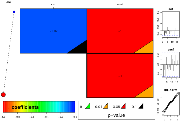
| Title produced by software | ARIMA Backward Selection | ||||||||||||||||||||||||||||||||||||||||||||||||||||||||||||||||||||||||||||||||||||||||||||||||||||||||||||||||||||||||||||||||||||||||||||||||||||||||||||||||||||||||||
| Date of computation | Sat, 06 Dec 2008 10:04:18 -0700 | ||||||||||||||||||||||||||||||||||||||||||||||||||||||||||||||||||||||||||||||||||||||||||||||||||||||||||||||||||||||||||||||||||||||||||||||||||||||||||||||||||||||||||
| Cite this page as follows | Statistical Computations at FreeStatistics.org, Office for Research Development and Education, URL https://freestatistics.org/blog/index.php?v=date/2008/Dec/06/t122858313987rxjsrpngcwdrf.htm/, Retrieved Sat, 18 May 2024 07:16:48 +0000 | ||||||||||||||||||||||||||||||||||||||||||||||||||||||||||||||||||||||||||||||||||||||||||||||||||||||||||||||||||||||||||||||||||||||||||||||||||||||||||||||||||||||||||
| Statistical Computations at FreeStatistics.org, Office for Research Development and Education, URL https://freestatistics.org/blog/index.php?pk=29757, Retrieved Sat, 18 May 2024 07:16:48 +0000 | |||||||||||||||||||||||||||||||||||||||||||||||||||||||||||||||||||||||||||||||||||||||||||||||||||||||||||||||||||||||||||||||||||||||||||||||||||||||||||||||||||||||||||
| QR Codes: | |||||||||||||||||||||||||||||||||||||||||||||||||||||||||||||||||||||||||||||||||||||||||||||||||||||||||||||||||||||||||||||||||||||||||||||||||||||||||||||||||||||||||||
|
| |||||||||||||||||||||||||||||||||||||||||||||||||||||||||||||||||||||||||||||||||||||||||||||||||||||||||||||||||||||||||||||||||||||||||||||||||||||||||||||||||||||||||||
| Original text written by user: | |||||||||||||||||||||||||||||||||||||||||||||||||||||||||||||||||||||||||||||||||||||||||||||||||||||||||||||||||||||||||||||||||||||||||||||||||||||||||||||||||||||||||||
| IsPrivate? | No (this computation is public) | ||||||||||||||||||||||||||||||||||||||||||||||||||||||||||||||||||||||||||||||||||||||||||||||||||||||||||||||||||||||||||||||||||||||||||||||||||||||||||||||||||||||||||
| User-defined keywords | |||||||||||||||||||||||||||||||||||||||||||||||||||||||||||||||||||||||||||||||||||||||||||||||||||||||||||||||||||||||||||||||||||||||||||||||||||||||||||||||||||||||||||
| Estimated Impact | 241 | ||||||||||||||||||||||||||||||||||||||||||||||||||||||||||||||||||||||||||||||||||||||||||||||||||||||||||||||||||||||||||||||||||||||||||||||||||||||||||||||||||||||||||
Tree of Dependent Computations | |||||||||||||||||||||||||||||||||||||||||||||||||||||||||||||||||||||||||||||||||||||||||||||||||||||||||||||||||||||||||||||||||||||||||||||||||||||||||||||||||||||||||||
| Family? (F = Feedback message, R = changed R code, M = changed R Module, P = changed Parameters, D = changed Data) | |||||||||||||||||||||||||||||||||||||||||||||||||||||||||||||||||||||||||||||||||||||||||||||||||||||||||||||||||||||||||||||||||||||||||||||||||||||||||||||||||||||||||||
| - [Univariate Data Series] [Run sequence plot...] [2008-12-02 22:19:27] [ed2ba3b6182103c15c0ab511ae4e6284] - RMPD [Standard Deviation-Mean Plot] [SD mean plot] [2008-12-06 11:49:39] [ed2ba3b6182103c15c0ab511ae4e6284] F RMP [(Partial) Autocorrelation Function] [ACF d=1 en D=1 la...] [2008-12-06 13:30:27] [ed2ba3b6182103c15c0ab511ae4e6284] - RM [ARIMA Backward Selection] [ARIMA model met q...] [2008-12-06 17:04:18] [c040f376c7eef5bfe1cb52dcc7980437] [Current] - P [ARIMA Backward Selection] [ARima backward se...] [2008-12-08 11:53:47] [ed2ba3b6182103c15c0ab511ae4e6284] - P [ARIMA Backward Selection] [MA controle] [2008-12-08 11:58:59] [ed2ba3b6182103c15c0ab511ae4e6284] F [ARIMA Backward Selection] [ARIMA] [2008-12-08 20:02:58] [4ad596f10399a71ad29b7d76e6ab90ac] - RMP [ARIMA Forecasting] [ARIMA forecast HI...] [2008-12-13 14:12:52] [ed2ba3b6182103c15c0ab511ae4e6284] - [ARIMA Backward Selection] [] [2008-12-08 21:34:29] [28075c6928548bea087cb2be962cfe7e] - P [ARIMA Backward Selection] [] [2008-12-09 00:38:49] [29747f79f5beb5b2516e1271770ecb47] - [ARIMA Backward Selection] [ARIMA] [2008-12-08 20:00:39] [4ad596f10399a71ad29b7d76e6ab90ac] F [ARIMA Backward Selection] [] [2008-12-08 21:33:18] [28075c6928548bea087cb2be962cfe7e] - [ARIMA Backward Selection] [Arima backward se...] [2008-12-09 00:33:34] [4ddbf81f78ea7c738951638c7e93f6ee] - P [ARIMA Backward Selection] [] [2008-12-09 00:36:36] [29747f79f5beb5b2516e1271770ecb47] - [ARIMA Backward Selection] [Arima backward se...] [2008-12-09 00:33:34] [4ddbf81f78ea7c738951638c7e93f6ee] F RMP [ARIMA Forecasting] [ARIMA forecasting] [2008-12-09 20:21:38] [ed2ba3b6182103c15c0ab511ae4e6284] F [ARIMA Forecasting] [Arima forecasting...] [2008-12-15 09:55:01] [4ad596f10399a71ad29b7d76e6ab90ac] F [ARIMA Forecasting] [ARIMA forecasting] [2008-12-15 09:56:32] [7506b5e9e41ec66c6657f4234f97306e] - [ARIMA Forecasting] [Arima Forecasting] [2008-12-15 10:39:39] [4ddbf81f78ea7c738951638c7e93f6ee] F [ARIMA Forecasting] [ARIMA] [2008-12-15 20:51:26] [28075c6928548bea087cb2be962cfe7e] F [ARIMA Forecasting] [arima forecasting] [2008-12-15 22:36:09] [005293453b571dbccb80b45226e44173] - [ARIMA Forecasting] [Forecasting] [2008-12-16 00:22:57] [c5e27150943bc3d623392efb0d98f8d3] | |||||||||||||||||||||||||||||||||||||||||||||||||||||||||||||||||||||||||||||||||||||||||||||||||||||||||||||||||||||||||||||||||||||||||||||||||||||||||||||||||||||||||||
| Feedback Forum | |||||||||||||||||||||||||||||||||||||||||||||||||||||||||||||||||||||||||||||||||||||||||||||||||||||||||||||||||||||||||||||||||||||||||||||||||||||||||||||||||||||||||||
Post a new message | |||||||||||||||||||||||||||||||||||||||||||||||||||||||||||||||||||||||||||||||||||||||||||||||||||||||||||||||||||||||||||||||||||||||||||||||||||||||||||||||||||||||||||
Dataset | |||||||||||||||||||||||||||||||||||||||||||||||||||||||||||||||||||||||||||||||||||||||||||||||||||||||||||||||||||||||||||||||||||||||||||||||||||||||||||||||||||||||||||
| Dataseries X: | |||||||||||||||||||||||||||||||||||||||||||||||||||||||||||||||||||||||||||||||||||||||||||||||||||||||||||||||||||||||||||||||||||||||||||||||||||||||||||||||||||||||||||
92.66 94.2 94.37 94.45 94.62 94.37 93.43 94.79 94.88 94.79 94.62 94.71 93.77 95.73 95.99 95.82 95.47 95.82 94.71 96.33 96.5 96.16 96.33 96.33 95.05 96.84 96.92 97.44 97.78 97.69 96.67 98.29 98.2 98.71 98.54 98.2 96.92 99.06 99.65 99.82 99.99 100.33 99.31 101.1 101.1 100.93 100.85 100.93 99.6 101.88 101.81 102.38 102.74 102.82 101.72 103.47 102.98 102.68 102.9 103.03 101.29 | |||||||||||||||||||||||||||||||||||||||||||||||||||||||||||||||||||||||||||||||||||||||||||||||||||||||||||||||||||||||||||||||||||||||||||||||||||||||||||||||||||||||||||
Tables (Output of Computation) | |||||||||||||||||||||||||||||||||||||||||||||||||||||||||||||||||||||||||||||||||||||||||||||||||||||||||||||||||||||||||||||||||||||||||||||||||||||||||||||||||||||||||||
| |||||||||||||||||||||||||||||||||||||||||||||||||||||||||||||||||||||||||||||||||||||||||||||||||||||||||||||||||||||||||||||||||||||||||||||||||||||||||||||||||||||||||||
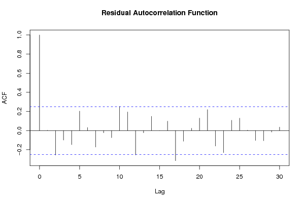
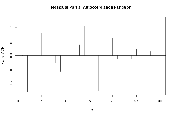
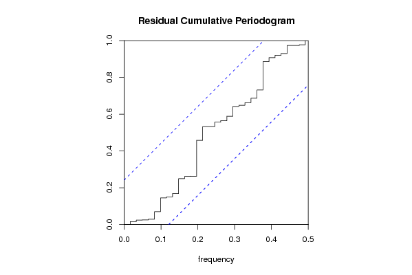
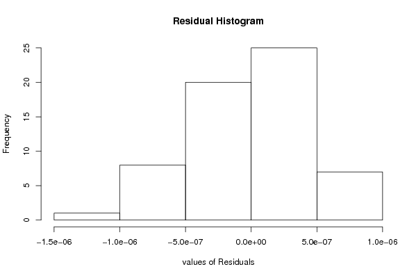
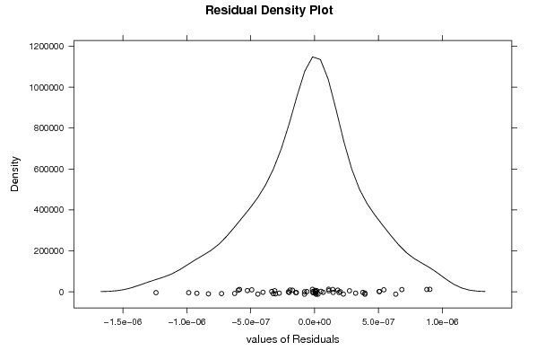
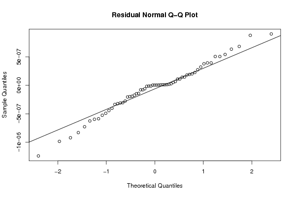
Figures (Output of Computation) | |||||||||||||||||||||||||||||||||||||||||||||||||||||||||||||||||||||||||||||||||||||||||||||||||||||||||||||||||||||||||||||||||||||||||||||||||||||||||||||||||||||||||||
Input Parameters & R Code | |||||||||||||||||||||||||||||||||||||||||||||||||||||||||||||||||||||||||||||||||||||||||||||||||||||||||||||||||||||||||||||||||||||||||||||||||||||||||||||||||||||||||||
| Parameters (Session): | |||||||||||||||||||||||||||||||||||||||||||||||||||||||||||||||||||||||||||||||||||||||||||||||||||||||||||||||||||||||||||||||||||||||||||||||||||||||||||||||||||||||||||
| par1 = 60 ; par2 = -2.0 ; par3 = 1 ; par4 = 1 ; par5 = 12 ; | |||||||||||||||||||||||||||||||||||||||||||||||||||||||||||||||||||||||||||||||||||||||||||||||||||||||||||||||||||||||||||||||||||||||||||||||||||||||||||||||||||||||||||
| Parameters (R input): | |||||||||||||||||||||||||||||||||||||||||||||||||||||||||||||||||||||||||||||||||||||||||||||||||||||||||||||||||||||||||||||||||||||||||||||||||||||||||||||||||||||||||||
| par1 = TRUE ; par2 = -2.0 ; par3 = 1 ; par4 = 1 ; par5 = 12 ; par6 = 0 ; par7 = 1 ; par8 = 0 ; par9 = 1 ; | |||||||||||||||||||||||||||||||||||||||||||||||||||||||||||||||||||||||||||||||||||||||||||||||||||||||||||||||||||||||||||||||||||||||||||||||||||||||||||||||||||||||||||
| R code (references can be found in the software module): | |||||||||||||||||||||||||||||||||||||||||||||||||||||||||||||||||||||||||||||||||||||||||||||||||||||||||||||||||||||||||||||||||||||||||||||||||||||||||||||||||||||||||||
library(lattice) | |||||||||||||||||||||||||||||||||||||||||||||||||||||||||||||||||||||||||||||||||||||||||||||||||||||||||||||||||||||||||||||||||||||||||||||||||||||||||||||||||||||||||||