Repository of Reproducible Computations

Free Statistics

of Irreproducible Research!

Author's title

Author

*Unverified author*

R Software Module

rwasp_autocorrelation.wasp

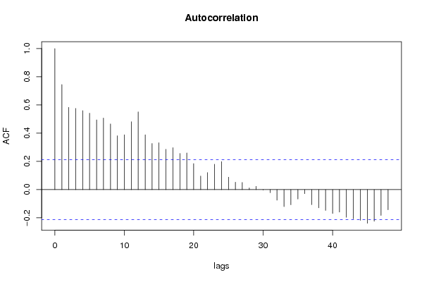
Title produced by software

(Partial) Autocorrelation Function

Date of computation

Tue, 09 Dec 2008 08:39:34 -0700

Cite this page as follows

Statistical Computations at FreeStatistics.org, Office for Research Development and Education, URL https://freestatistics.org/blog/index.php?v=date/2008/Dec/09/t1228837246m916tub0k2upxi8.htm/, Retrieved Sat, 18 May 2024 08:26:26 +0000

Statistical Computations at FreeStatistics.org, Office for Research Development and Education, URL https://freestatistics.org/blog/index.php?pk=31523, Retrieved Sat, 18 May 2024 08:26:26 +0000

QR Codes:

Paste this QR Code to cite your computation.

Original text written by user:

IsPrivate?

No (this computation is public)

User-defined keywords

Estimated Impact

196

Family? (F = Feedback message, R = changed R code, M = changed R Module, P = changed Parameters, D = changed Data)

F       [(Partial) Autocorrelation Function] [step acf] [2008-12-09 15:39:34] [d41d8cd98f00b204e9800998ecf8427e] [Current]
F RMP     [Variance Reduction Matrix] [step 2 vrm] [2008-12-09 18:16:38] [74be16979710d4c4e7c6647856088456] 
F RMP     [Spectral Analysis] [step 2 spectral] [2008-12-09 18:22:37] [74be16979710d4c4e7c6647856088456] 
-   P     [(Partial) Autocorrelation Function] [step 3 acf] [2008-12-09 18:41:47] [74be16979710d4c4e7c6647856088456] 
-   P       [(Partial) Autocorrelation Function] [step 2 met d=0] [2008-12-11 10:51:35] [74be16979710d4c4e7c6647856088456] 
- RMP       [Spectral Analysis] [step 2 met d=0 sp...] [2008-12-11 10:50:31] [74be16979710d4c4e7c6647856088456] 
-   P       [(Partial) Autocorrelation Function] [sdsdsd] [2008-12-11 11:20:34] [74be16979710d4c4e7c6647856088456] 
- RMP     [Spectral Analysis] [] [2008-12-09 18:44:40] [74be16979710d4c4e7c6647856088456] 
F   PD    [(Partial) Autocorrelation Function] [step 2 airline] [2008-12-09 19:04:41] [74be16979710d4c4e7c6647856088456] 
F RMPD    [ARIMA Backward Selection] [step 5 unemployme...] [2008-12-09 19:25:52] [74be16979710d4c4e7c6647856088456] 

Feedback Forum

2008-12-15 15:33:11 [c00776cbed2786c9c4960950021bd861] [reply] 
Er is inderdaad een lange termijntrend te zien. (of deze duidelijk is, is relatief..) Ook de invloed van seizoenaliteit is vast te stellen, zoals de student(e) heeft opgemerkt. 
We moeten dus de d en D gelijkstellen aan 1.

Post a new message

Dataseries X:

Download CSV

Histogram

Boxplots

Summary of computational transaction
Raw Input	view raw input (R code)
Raw Output	view raw output of R engine
Computing time	3 seconds
R Server	'George Udny Yule' @ 72.249.76.132

\begin{tabular}{lllllllll}
\hline
Summary of computational transaction \tabularnewline
Raw Input & view raw input (R code)  \tabularnewline
Raw Output & view raw output of R engine  \tabularnewline
Computing time & 3 seconds \tabularnewline
R Server & 'George Udny Yule' @ 72.249.76.132 \tabularnewline
\hline
\end{tabular}
%Source: https://freestatistics.org/blog/index.php?pk=31523&T=0

[TABLE]
[ROW][C]Summary of computational transaction[/C][/ROW]
[ROW][C]Raw Input[/C][C]view raw input (R code) [/C][/ROW]
[ROW][C]Raw Output[/C][C]view raw output of R engine [/C][/ROW]
[ROW][C]Computing time[/C][C]3 seconds[/C][/ROW]
[ROW][C]R Server[/C][C]'George Udny Yule' @ 72.249.76.132[/C][/ROW]
[/TABLE]
Source: https://freestatistics.org/blog/index.php?pk=31523&T=0

Globally Unique Identifier (entire table): ba.freestatistics.org/blog/index.php?pk=31523&T=0

As an alternative you can also use a QR Code:

The GUIDs for individual cells are displayed in the table below:

Summary of computational transaction
Raw Input	view raw input (R code)
Raw Output	view raw output of R engine
Computing time	3 seconds
R Server	'George Udny Yule' @ 72.249.76.132

Autocorrelation Function
Time lag k	ACF(k)	T-STAT	P-value
1	0.745102	6.8695	0
2	0.583457	5.3792	0
3	0.575582	5.3066	0
4	0.560272	5.1655	1e-06
5	0.542115	4.9981	2e-06
6	0.494424	4.5584	9e-06
7	0.507284	4.6769	5e-06
8	0.465768	4.2942	2.3e-05
9	0.381882	3.5208	0.000347
10	0.388845	3.585	0.000281
11	0.481135	4.4358	1.4e-05
12	0.551579	5.0853	1e-06
13	0.389072	3.5871	0.000279
14	0.327073	3.0155	0.001691
15	0.332572	3.0662	0.001453
16	0.285748	2.6345	0.005006
17	0.297836	2.7459	0.003682
18	0.256548	2.3653	0.010147
19	0.260342	2.4002	0.009284
20	0.184217	1.6984	0.046546
21	0.096342	0.8882	0.188462
22	0.120977	1.1154	0.133921
23	0.180241	1.6617	0.050125
24	0.198739	1.8323	0.035206
25	0.08811	0.8123	0.209433
26	0.052789	0.4867	0.313866
27	0.050654	0.467	0.320843
28	0.011866	0.1094	0.45657
29	0.02295	0.2116	0.416468
30	-0.002971	-0.0274	0.489106
31	-0.021534	-0.1985	0.421552
32	-0.074862	-0.6902	0.245976
33	-0.120373	-1.1098	0.135111
34	-0.107161	-0.988	0.162984
35	-0.066752	-0.6154	0.269961
36	-0.028742	-0.265	0.395829
37	-0.106916	-0.9857	0.163534
38	-0.129588	-1.1947	0.117755
39	-0.14772	-1.3619	0.088413
40	-0.169533	-1.563	0.060882
41	-0.159533	-1.4708	0.072516
42	-0.196477	-1.8114	0.036803
43	-0.206788	-1.9065	0.029983
44	-0.217972	-2.0096	0.023823
45	-0.238476	-2.1986	0.01531
46	-0.224553	-2.0703	0.020731
47	-0.183244	-1.6894	0.047402
48	-0.143106	-1.3194	0.095294

\begin{tabular}{lllllllll}
\hline
Autocorrelation Function \tabularnewline
Time lag k & ACF(k) & T-STAT & P-value \tabularnewline
1 & 0.745102 & 6.8695 & 0 \tabularnewline
2 & 0.583457 & 5.3792 & 0 \tabularnewline
3 & 0.575582 & 5.3066 & 0 \tabularnewline
4 & 0.560272 & 5.1655 & 1e-06 \tabularnewline
5 & 0.542115 & 4.9981 & 2e-06 \tabularnewline
6 & 0.494424 & 4.5584 & 9e-06 \tabularnewline
7 & 0.507284 & 4.6769 & 5e-06 \tabularnewline
8 & 0.465768 & 4.2942 & 2.3e-05 \tabularnewline
9 & 0.381882 & 3.5208 & 0.000347 \tabularnewline
10 & 0.388845 & 3.585 & 0.000281 \tabularnewline
11 & 0.481135 & 4.4358 & 1.4e-05 \tabularnewline
12 & 0.551579 & 5.0853 & 1e-06 \tabularnewline
13 & 0.389072 & 3.5871 & 0.000279 \tabularnewline
14 & 0.327073 & 3.0155 & 0.001691 \tabularnewline
15 & 0.332572 & 3.0662 & 0.001453 \tabularnewline
16 & 0.285748 & 2.6345 & 0.005006 \tabularnewline
17 & 0.297836 & 2.7459 & 0.003682 \tabularnewline
18 & 0.256548 & 2.3653 & 0.010147 \tabularnewline
19 & 0.260342 & 2.4002 & 0.009284 \tabularnewline
20 & 0.184217 & 1.6984 & 0.046546 \tabularnewline
21 & 0.096342 & 0.8882 & 0.188462 \tabularnewline
22 & 0.120977 & 1.1154 & 0.133921 \tabularnewline
23 & 0.180241 & 1.6617 & 0.050125 \tabularnewline
24 & 0.198739 & 1.8323 & 0.035206 \tabularnewline
25 & 0.08811 & 0.8123 & 0.209433 \tabularnewline
26 & 0.052789 & 0.4867 & 0.313866 \tabularnewline
27 & 0.050654 & 0.467 & 0.320843 \tabularnewline
28 & 0.011866 & 0.1094 & 0.45657 \tabularnewline
29 & 0.02295 & 0.2116 & 0.416468 \tabularnewline
30 & -0.002971 & -0.0274 & 0.489106 \tabularnewline
31 & -0.021534 & -0.1985 & 0.421552 \tabularnewline
32 & -0.074862 & -0.6902 & 0.245976 \tabularnewline
33 & -0.120373 & -1.1098 & 0.135111 \tabularnewline
34 & -0.107161 & -0.988 & 0.162984 \tabularnewline
35 & -0.066752 & -0.6154 & 0.269961 \tabularnewline
36 & -0.028742 & -0.265 & 0.395829 \tabularnewline
37 & -0.106916 & -0.9857 & 0.163534 \tabularnewline
38 & -0.129588 & -1.1947 & 0.117755 \tabularnewline
39 & -0.14772 & -1.3619 & 0.088413 \tabularnewline
40 & -0.169533 & -1.563 & 0.060882 \tabularnewline
41 & -0.159533 & -1.4708 & 0.072516 \tabularnewline
42 & -0.196477 & -1.8114 & 0.036803 \tabularnewline
43 & -0.206788 & -1.9065 & 0.029983 \tabularnewline
44 & -0.217972 & -2.0096 & 0.023823 \tabularnewline
45 & -0.238476 & -2.1986 & 0.01531 \tabularnewline
46 & -0.224553 & -2.0703 & 0.020731 \tabularnewline
47 & -0.183244 & -1.6894 & 0.047402 \tabularnewline
48 & -0.143106 & -1.3194 & 0.095294 \tabularnewline
\hline
\end{tabular}
%Source: https://freestatistics.org/blog/index.php?pk=31523&T=1

[TABLE]
[ROW][C]Autocorrelation Function[/C][/ROW]
[ROW][C]Time lag k[/C][C]ACF(k)[/C][C]T-STAT[/C][C]P-value[/C][/ROW]
[ROW][C]1[/C][C]0.745102[/C][C]6.8695[/C][C]0[/C][/ROW]
[ROW][C]2[/C][C]0.583457[/C][C]5.3792[/C][C]0[/C][/ROW]
[ROW][C]3[/C][C]0.575582[/C][C]5.3066[/C][C]0[/C][/ROW]
[ROW][C]4[/C][C]0.560272[/C][C]5.1655[/C][C]1e-06[/C][/ROW]
[ROW][C]5[/C][C]0.542115[/C][C]4.9981[/C][C]2e-06[/C][/ROW]
[ROW][C]6[/C][C]0.494424[/C][C]4.5584[/C][C]9e-06[/C][/ROW]
[ROW][C]7[/C][C]0.507284[/C][C]4.6769[/C][C]5e-06[/C][/ROW]
[ROW][C]8[/C][C]0.465768[/C][C]4.2942[/C][C]2.3e-05[/C][/ROW]
[ROW][C]9[/C][C]0.381882[/C][C]3.5208[/C][C]0.000347[/C][/ROW]
[ROW][C]10[/C][C]0.388845[/C][C]3.585[/C][C]0.000281[/C][/ROW]
[ROW][C]11[/C][C]0.481135[/C][C]4.4358[/C][C]1.4e-05[/C][/ROW]
[ROW][C]12[/C][C]0.551579[/C][C]5.0853[/C][C]1e-06[/C][/ROW]
[ROW][C]13[/C][C]0.389072[/C][C]3.5871[/C][C]0.000279[/C][/ROW]
[ROW][C]14[/C][C]0.327073[/C][C]3.0155[/C][C]0.001691[/C][/ROW]
[ROW][C]15[/C][C]0.332572[/C][C]3.0662[/C][C]0.001453[/C][/ROW]
[ROW][C]16[/C][C]0.285748[/C][C]2.6345[/C][C]0.005006[/C][/ROW]
[ROW][C]17[/C][C]0.297836[/C][C]2.7459[/C][C]0.003682[/C][/ROW]
[ROW][C]18[/C][C]0.256548[/C][C]2.3653[/C][C]0.010147[/C][/ROW]
[ROW][C]19[/C][C]0.260342[/C][C]2.4002[/C][C]0.009284[/C][/ROW]
[ROW][C]20[/C][C]0.184217[/C][C]1.6984[/C][C]0.046546[/C][/ROW]
[ROW][C]21[/C][C]0.096342[/C][C]0.8882[/C][C]0.188462[/C][/ROW]
[ROW][C]22[/C][C]0.120977[/C][C]1.1154[/C][C]0.133921[/C][/ROW]
[ROW][C]23[/C][C]0.180241[/C][C]1.6617[/C][C]0.050125[/C][/ROW]
[ROW][C]24[/C][C]0.198739[/C][C]1.8323[/C][C]0.035206[/C][/ROW]
[ROW][C]25[/C][C]0.08811[/C][C]0.8123[/C][C]0.209433[/C][/ROW]
[ROW][C]26[/C][C]0.052789[/C][C]0.4867[/C][C]0.313866[/C][/ROW]
[ROW][C]27[/C][C]0.050654[/C][C]0.467[/C][C]0.320843[/C][/ROW]
[ROW][C]28[/C][C]0.011866[/C][C]0.1094[/C][C]0.45657[/C][/ROW]
[ROW][C]29[/C][C]0.02295[/C][C]0.2116[/C][C]0.416468[/C][/ROW]
[ROW][C]30[/C][C]-0.002971[/C][C]-0.0274[/C][C]0.489106[/C][/ROW]
[ROW][C]31[/C][C]-0.021534[/C][C]-0.1985[/C][C]0.421552[/C][/ROW]
[ROW][C]32[/C][C]-0.074862[/C][C]-0.6902[/C][C]0.245976[/C][/ROW]
[ROW][C]33[/C][C]-0.120373[/C][C]-1.1098[/C][C]0.135111[/C][/ROW]
[ROW][C]34[/C][C]-0.107161[/C][C]-0.988[/C][C]0.162984[/C][/ROW]
[ROW][C]35[/C][C]-0.066752[/C][C]-0.6154[/C][C]0.269961[/C][/ROW]
[ROW][C]36[/C][C]-0.028742[/C][C]-0.265[/C][C]0.395829[/C][/ROW]
[ROW][C]37[/C][C]-0.106916[/C][C]-0.9857[/C][C]0.163534[/C][/ROW]
[ROW][C]38[/C][C]-0.129588[/C][C]-1.1947[/C][C]0.117755[/C][/ROW]
[ROW][C]39[/C][C]-0.14772[/C][C]-1.3619[/C][C]0.088413[/C][/ROW]
[ROW][C]40[/C][C]-0.169533[/C][C]-1.563[/C][C]0.060882[/C][/ROW]
[ROW][C]41[/C][C]-0.159533[/C][C]-1.4708[/C][C]0.072516[/C][/ROW]
[ROW][C]42[/C][C]-0.196477[/C][C]-1.8114[/C][C]0.036803[/C][/ROW]
[ROW][C]43[/C][C]-0.206788[/C][C]-1.9065[/C][C]0.029983[/C][/ROW]
[ROW][C]44[/C][C]-0.217972[/C][C]-2.0096[/C][C]0.023823[/C][/ROW]
[ROW][C]45[/C][C]-0.238476[/C][C]-2.1986[/C][C]0.01531[/C][/ROW]
[ROW][C]46[/C][C]-0.224553[/C][C]-2.0703[/C][C]0.020731[/C][/ROW]
[ROW][C]47[/C][C]-0.183244[/C][C]-1.6894[/C][C]0.047402[/C][/ROW]
[ROW][C]48[/C][C]-0.143106[/C][C]-1.3194[/C][C]0.095294[/C][/ROW]
[/TABLE]
Source: https://freestatistics.org/blog/index.php?pk=31523&T=1

Globally Unique Identifier (entire table): ba.freestatistics.org/blog/index.php?pk=31523&T=1

As an alternative you can also use a QR Code:

The GUIDs for individual cells are displayed in the table below:

Autocorrelation Function
Time lag k	ACF(k)	T-STAT	P-value
1	0.745102	6.8695	0
2	0.583457	5.3792	0
3	0.575582	5.3066	0
4	0.560272	5.1655	1e-06
5	0.542115	4.9981	2e-06
6	0.494424	4.5584	9e-06
7	0.507284	4.6769	5e-06
8	0.465768	4.2942	2.3e-05
9	0.381882	3.5208	0.000347
10	0.388845	3.585	0.000281
11	0.481135	4.4358	1.4e-05
12	0.551579	5.0853	1e-06
13	0.389072	3.5871	0.000279
14	0.327073	3.0155	0.001691
15	0.332572	3.0662	0.001453
16	0.285748	2.6345	0.005006
17	0.297836	2.7459	0.003682
18	0.256548	2.3653	0.010147
19	0.260342	2.4002	0.009284
20	0.184217	1.6984	0.046546
21	0.096342	0.8882	0.188462
22	0.120977	1.1154	0.133921
23	0.180241	1.6617	0.050125
24	0.198739	1.8323	0.035206
25	0.08811	0.8123	0.209433
26	0.052789	0.4867	0.313866
27	0.050654	0.467	0.320843
28	0.011866	0.1094	0.45657
29	0.02295	0.2116	0.416468
30	-0.002971	-0.0274	0.489106
31	-0.021534	-0.1985	0.421552
32	-0.074862	-0.6902	0.245976
33	-0.120373	-1.1098	0.135111
34	-0.107161	-0.988	0.162984
35	-0.066752	-0.6154	0.269961
36	-0.028742	-0.265	0.395829
37	-0.106916	-0.9857	0.163534
38	-0.129588	-1.1947	0.117755
39	-0.14772	-1.3619	0.088413
40	-0.169533	-1.563	0.060882
41	-0.159533	-1.4708	0.072516
42	-0.196477	-1.8114	0.036803
43	-0.206788	-1.9065	0.029983
44	-0.217972	-2.0096	0.023823
45	-0.238476	-2.1986	0.01531
46	-0.224553	-2.0703	0.020731
47	-0.183244	-1.6894	0.047402
48	-0.143106	-1.3194	0.095294

Partial Autocorrelation Function
Time lag k	PACF(k)	T-STAT	P-value
1	0.745102	6.8695	0
2	0.063577	0.5862	0.279664
3	0.273382	2.5205	0.006794
4	0.095571	0.8811	0.190369
5	0.120626	1.1121	0.134612
6	-0.007442	-0.0686	0.472731
7	0.157251	1.4498	0.0754
8	-0.076919	-0.7092	0.240084
9	-0.07304	-0.6734	0.251263
10	0.081696	0.7532	0.226706
11	0.239889	2.2117	0.014836
12	0.193486	1.7839	0.039008
13	-0.344379	-3.175	0.001044
14	0.036139	0.3332	0.369909
15	-0.091189	-0.8407	0.201432
16	-0.048547	-0.4476	0.327797
17	0.082149	0.7574	0.225459
18	-0.126435	-1.1657	0.123504
19	0.047413	0.4371	0.331565
20	-0.14901	-1.3738	0.086558
21	0.003665	0.0338	0.486562
22	-0.046339	-0.4272	0.335149
23	0.071762	0.6616	0.255004
24	0.012795	0.118	0.453186
25	-0.097094	-0.8952	0.186614
26	0.003424	0.0316	0.487444
27	-0.062138	-0.5729	0.284119
28	0.0321	0.296	0.383995
29	-0.068887	-0.6351	0.263534
30	-0.004619	-0.0426	0.483066
31	-0.0808	-0.7449	0.229182
32	0.048945	0.4513	0.326478
33	0.034099	0.3144	0.377003
34	-0.121917	-1.124	0.132084
35	0.108861	1.0036	0.159198
36	0.029414	0.2712	0.393453
37	-0.039346	-0.3627	0.358846
38	-0.005985	-0.0552	0.478061
39	-0.092082	-0.849	0.199145
40	0.028348	0.2614	0.397225
41	-0.094661	-0.8727	0.192634
42	-0.012805	-0.1181	0.453152
43	-0.047097	-0.4342	0.332617
44	0.089515	0.8253	0.20576
45	0.025008	0.2306	0.409103
46	-0.025999	-0.2397	0.405569
47	0.035678	0.3289	0.371508
48	-0.002094	-0.0193	0.49232

\begin{tabular}{lllllllll}
\hline
Partial Autocorrelation Function \tabularnewline
Time lag k & PACF(k) & T-STAT & P-value \tabularnewline
1 & 0.745102 & 6.8695 & 0 \tabularnewline
2 & 0.063577 & 0.5862 & 0.279664 \tabularnewline
3 & 0.273382 & 2.5205 & 0.006794 \tabularnewline
4 & 0.095571 & 0.8811 & 0.190369 \tabularnewline
5 & 0.120626 & 1.1121 & 0.134612 \tabularnewline
6 & -0.007442 & -0.0686 & 0.472731 \tabularnewline
7 & 0.157251 & 1.4498 & 0.0754 \tabularnewline
8 & -0.076919 & -0.7092 & 0.240084 \tabularnewline
9 & -0.07304 & -0.6734 & 0.251263 \tabularnewline
10 & 0.081696 & 0.7532 & 0.226706 \tabularnewline
11 & 0.239889 & 2.2117 & 0.014836 \tabularnewline
12 & 0.193486 & 1.7839 & 0.039008 \tabularnewline
13 & -0.344379 & -3.175 & 0.001044 \tabularnewline
14 & 0.036139 & 0.3332 & 0.369909 \tabularnewline
15 & -0.091189 & -0.8407 & 0.201432 \tabularnewline
16 & -0.048547 & -0.4476 & 0.327797 \tabularnewline
17 & 0.082149 & 0.7574 & 0.225459 \tabularnewline
18 & -0.126435 & -1.1657 & 0.123504 \tabularnewline
19 & 0.047413 & 0.4371 & 0.331565 \tabularnewline
20 & -0.14901 & -1.3738 & 0.086558 \tabularnewline
21 & 0.003665 & 0.0338 & 0.486562 \tabularnewline
22 & -0.046339 & -0.4272 & 0.335149 \tabularnewline
23 & 0.071762 & 0.6616 & 0.255004 \tabularnewline
24 & 0.012795 & 0.118 & 0.453186 \tabularnewline
25 & -0.097094 & -0.8952 & 0.186614 \tabularnewline
26 & 0.003424 & 0.0316 & 0.487444 \tabularnewline
27 & -0.062138 & -0.5729 & 0.284119 \tabularnewline
28 & 0.0321 & 0.296 & 0.383995 \tabularnewline
29 & -0.068887 & -0.6351 & 0.263534 \tabularnewline
30 & -0.004619 & -0.0426 & 0.483066 \tabularnewline
31 & -0.0808 & -0.7449 & 0.229182 \tabularnewline
32 & 0.048945 & 0.4513 & 0.326478 \tabularnewline
33 & 0.034099 & 0.3144 & 0.377003 \tabularnewline
34 & -0.121917 & -1.124 & 0.132084 \tabularnewline
35 & 0.108861 & 1.0036 & 0.159198 \tabularnewline
36 & 0.029414 & 0.2712 & 0.393453 \tabularnewline
37 & -0.039346 & -0.3627 & 0.358846 \tabularnewline
38 & -0.005985 & -0.0552 & 0.478061 \tabularnewline
39 & -0.092082 & -0.849 & 0.199145 \tabularnewline
40 & 0.028348 & 0.2614 & 0.397225 \tabularnewline
41 & -0.094661 & -0.8727 & 0.192634 \tabularnewline
42 & -0.012805 & -0.1181 & 0.453152 \tabularnewline
43 & -0.047097 & -0.4342 & 0.332617 \tabularnewline
44 & 0.089515 & 0.8253 & 0.20576 \tabularnewline
45 & 0.025008 & 0.2306 & 0.409103 \tabularnewline
46 & -0.025999 & -0.2397 & 0.405569 \tabularnewline
47 & 0.035678 & 0.3289 & 0.371508 \tabularnewline
48 & -0.002094 & -0.0193 & 0.49232 \tabularnewline
\hline
\end{tabular}
%Source: https://freestatistics.org/blog/index.php?pk=31523&T=2

[TABLE]
[ROW][C]Partial Autocorrelation Function[/C][/ROW]
[ROW][C]Time lag k[/C][C]PACF(k)[/C][C]T-STAT[/C][C]P-value[/C][/ROW]
[ROW][C]1[/C][C]0.745102[/C][C]6.8695[/C][C]0[/C][/ROW]
[ROW][C]2[/C][C]0.063577[/C][C]0.5862[/C][C]0.279664[/C][/ROW]
[ROW][C]3[/C][C]0.273382[/C][C]2.5205[/C][C]0.006794[/C][/ROW]
[ROW][C]4[/C][C]0.095571[/C][C]0.8811[/C][C]0.190369[/C][/ROW]
[ROW][C]5[/C][C]0.120626[/C][C]1.1121[/C][C]0.134612[/C][/ROW]
[ROW][C]6[/C][C]-0.007442[/C][C]-0.0686[/C][C]0.472731[/C][/ROW]
[ROW][C]7[/C][C]0.157251[/C][C]1.4498[/C][C]0.0754[/C][/ROW]
[ROW][C]8[/C][C]-0.076919[/C][C]-0.7092[/C][C]0.240084[/C][/ROW]
[ROW][C]9[/C][C]-0.07304[/C][C]-0.6734[/C][C]0.251263[/C][/ROW]
[ROW][C]10[/C][C]0.081696[/C][C]0.7532[/C][C]0.226706[/C][/ROW]
[ROW][C]11[/C][C]0.239889[/C][C]2.2117[/C][C]0.014836[/C][/ROW]
[ROW][C]12[/C][C]0.193486[/C][C]1.7839[/C][C]0.039008[/C][/ROW]
[ROW][C]13[/C][C]-0.344379[/C][C]-3.175[/C][C]0.001044[/C][/ROW]
[ROW][C]14[/C][C]0.036139[/C][C]0.3332[/C][C]0.369909[/C][/ROW]
[ROW][C]15[/C][C]-0.091189[/C][C]-0.8407[/C][C]0.201432[/C][/ROW]
[ROW][C]16[/C][C]-0.048547[/C][C]-0.4476[/C][C]0.327797[/C][/ROW]
[ROW][C]17[/C][C]0.082149[/C][C]0.7574[/C][C]0.225459[/C][/ROW]
[ROW][C]18[/C][C]-0.126435[/C][C]-1.1657[/C][C]0.123504[/C][/ROW]
[ROW][C]19[/C][C]0.047413[/C][C]0.4371[/C][C]0.331565[/C][/ROW]
[ROW][C]20[/C][C]-0.14901[/C][C]-1.3738[/C][C]0.086558[/C][/ROW]
[ROW][C]21[/C][C]0.003665[/C][C]0.0338[/C][C]0.486562[/C][/ROW]
[ROW][C]22[/C][C]-0.046339[/C][C]-0.4272[/C][C]0.335149[/C][/ROW]
[ROW][C]23[/C][C]0.071762[/C][C]0.6616[/C][C]0.255004[/C][/ROW]
[ROW][C]24[/C][C]0.012795[/C][C]0.118[/C][C]0.453186[/C][/ROW]
[ROW][C]25[/C][C]-0.097094[/C][C]-0.8952[/C][C]0.186614[/C][/ROW]
[ROW][C]26[/C][C]0.003424[/C][C]0.0316[/C][C]0.487444[/C][/ROW]
[ROW][C]27[/C][C]-0.062138[/C][C]-0.5729[/C][C]0.284119[/C][/ROW]
[ROW][C]28[/C][C]0.0321[/C][C]0.296[/C][C]0.383995[/C][/ROW]
[ROW][C]29[/C][C]-0.068887[/C][C]-0.6351[/C][C]0.263534[/C][/ROW]
[ROW][C]30[/C][C]-0.004619[/C][C]-0.0426[/C][C]0.483066[/C][/ROW]
[ROW][C]31[/C][C]-0.0808[/C][C]-0.7449[/C][C]0.229182[/C][/ROW]
[ROW][C]32[/C][C]0.048945[/C][C]0.4513[/C][C]0.326478[/C][/ROW]
[ROW][C]33[/C][C]0.034099[/C][C]0.3144[/C][C]0.377003[/C][/ROW]
[ROW][C]34[/C][C]-0.121917[/C][C]-1.124[/C][C]0.132084[/C][/ROW]
[ROW][C]35[/C][C]0.108861[/C][C]1.0036[/C][C]0.159198[/C][/ROW]
[ROW][C]36[/C][C]0.029414[/C][C]0.2712[/C][C]0.393453[/C][/ROW]
[ROW][C]37[/C][C]-0.039346[/C][C]-0.3627[/C][C]0.358846[/C][/ROW]
[ROW][C]38[/C][C]-0.005985[/C][C]-0.0552[/C][C]0.478061[/C][/ROW]
[ROW][C]39[/C][C]-0.092082[/C][C]-0.849[/C][C]0.199145[/C][/ROW]
[ROW][C]40[/C][C]0.028348[/C][C]0.2614[/C][C]0.397225[/C][/ROW]
[ROW][C]41[/C][C]-0.094661[/C][C]-0.8727[/C][C]0.192634[/C][/ROW]
[ROW][C]42[/C][C]-0.012805[/C][C]-0.1181[/C][C]0.453152[/C][/ROW]
[ROW][C]43[/C][C]-0.047097[/C][C]-0.4342[/C][C]0.332617[/C][/ROW]
[ROW][C]44[/C][C]0.089515[/C][C]0.8253[/C][C]0.20576[/C][/ROW]
[ROW][C]45[/C][C]0.025008[/C][C]0.2306[/C][C]0.409103[/C][/ROW]
[ROW][C]46[/C][C]-0.025999[/C][C]-0.2397[/C][C]0.405569[/C][/ROW]
[ROW][C]47[/C][C]0.035678[/C][C]0.3289[/C][C]0.371508[/C][/ROW]
[ROW][C]48[/C][C]-0.002094[/C][C]-0.0193[/C][C]0.49232[/C][/ROW]
[/TABLE]
Source: https://freestatistics.org/blog/index.php?pk=31523&T=2

Globally Unique Identifier (entire table): ba.freestatistics.org/blog/index.php?pk=31523&T=2

As an alternative you can also use a QR Code:

The GUIDs for individual cells are displayed in the table below:

Partial Autocorrelation Function
Time lag k	PACF(k)	T-STAT	P-value
1	0.745102	6.8695	0
2	0.063577	0.5862	0.279664
3	0.273382	2.5205	0.006794
4	0.095571	0.8811	0.190369
5	0.120626	1.1121	0.134612
6	-0.007442	-0.0686	0.472731
7	0.157251	1.4498	0.0754
8	-0.076919	-0.7092	0.240084
9	-0.07304	-0.6734	0.251263
10	0.081696	0.7532	0.226706
11	0.239889	2.2117	0.014836
12	0.193486	1.7839	0.039008
13	-0.344379	-3.175	0.001044
14	0.036139	0.3332	0.369909
15	-0.091189	-0.8407	0.201432
16	-0.048547	-0.4476	0.327797
17	0.082149	0.7574	0.225459
18	-0.126435	-1.1657	0.123504
19	0.047413	0.4371	0.331565
20	-0.14901	-1.3738	0.086558
21	0.003665	0.0338	0.486562
22	-0.046339	-0.4272	0.335149
23	0.071762	0.6616	0.255004
24	0.012795	0.118	0.453186
25	-0.097094	-0.8952	0.186614
26	0.003424	0.0316	0.487444
27	-0.062138	-0.5729	0.284119
28	0.0321	0.296	0.383995
29	-0.068887	-0.6351	0.263534
30	-0.004619	-0.0426	0.483066
31	-0.0808	-0.7449	0.229182
32	0.048945	0.4513	0.326478
33	0.034099	0.3144	0.377003
34	-0.121917	-1.124	0.132084
35	0.108861	1.0036	0.159198
36	0.029414	0.2712	0.393453
37	-0.039346	-0.3627	0.358846
38	-0.005985	-0.0552	0.478061
39	-0.092082	-0.849	0.199145
40	0.028348	0.2614	0.397225
41	-0.094661	-0.8727	0.192634
42	-0.012805	-0.1181	0.453152
43	-0.047097	-0.4342	0.332617
44	0.089515	0.8253	0.20576
45	0.025008	0.2306	0.409103
46	-0.025999	-0.2397	0.405569
47	0.035678	0.3289	0.371508
48	-0.002094	-0.0193	0.49232

Figure 1

PNG link

Postscript link

PDF link

Figure 2

PNG link

Postscript link

PDF link

Parameters (Session):

par1 = 48 ; par2 = 1 ; par3 = 0 ; par4 = 0 ; par5 = 12 ;

Parameters (R input):

par1 = 48 ; par2 = 1 ; par3 = 0 ; par4 = 0 ; par5 = 12 ;

R code (references can be found in the software module):

if (par1 == 'Default') {
par1 = 10*log10(length(x))
} else {
par1 <- as.numeric(par1)
}
par2 <- as.numeric(par2)
par3 <- as.numeric(par3)
par4 <- as.numeric(par4)
par5 <- as.numeric(par5)
if (par2 == 0) {
x <- log(x)
} else {
x <- (x ^ par2 - 1) / par2
}
if (par3 > 0) x <- diff(x,lag=1,difference=par3)
if (par4 > 0) x <- diff(x,lag=par5,difference=par4)
bitmap(file='pic1.png')
racf <- acf(x,par1,main='Autocorrelation',xlab='lags',ylab='ACF')
dev.off()
bitmap(file='pic2.png')
rpacf <- pacf(x,par1,main='Partial Autocorrelation',xlab='lags',ylab='PACF')
dev.off()
(myacf <- c(racf$acf))
(mypacf <- c(rpacf$acf))
lengthx <- length(x)
sqrtn <- sqrt(lengthx)
load(file='createtable')
a<-table.start()
a<-table.row.start(a)
a<-table.element(a,'Autocorrelation Function',4,TRUE)
a<-table.row.end(a)
a<-table.row.start(a)
a<-table.element(a,'Time lag k',header=TRUE)
a<-table.element(a,hyperlink('basics.htm','ACF(k)','click here for more information about the Autocorrelation Function'),header=TRUE)
a<-table.element(a,'T-STAT',header=TRUE)
a<-table.element(a,'P-value',header=TRUE)
a<-table.row.end(a)
for (i in 2:(par1+1)) {
a<-table.row.start(a)
a<-table.element(a,i-1,header=TRUE)
a<-table.element(a,round(myacf[i],6))
mytstat <- myacf[i]*sqrtn
a<-table.element(a,round(mytstat,4))
a<-table.element(a,round(1-pt(abs(mytstat),lengthx),6))
a<-table.row.end(a)
}
a<-table.end(a)
table.save(a,file='mytable.tab')
a<-table.start()
a<-table.row.start(a)
a<-table.element(a,'Partial Autocorrelation Function',4,TRUE)
a<-table.row.end(a)
a<-table.row.start(a)
a<-table.element(a,'Time lag k',header=TRUE)
a<-table.element(a,hyperlink('basics.htm','PACF(k)','click here for more information about the Partial Autocorrelation Function'),header=TRUE)
a<-table.element(a,'T-STAT',header=TRUE)
a<-table.element(a,'P-value',header=TRUE)
a<-table.row.end(a)
for (i in 1:par1) {
a<-table.row.start(a)
a<-table.element(a,i,header=TRUE)
a<-table.element(a,round(mypacf[i],6))
mytstat <- mypacf[i]*sqrtn
a<-table.element(a,round(mytstat,4))
a<-table.element(a,round(1-pt(abs(mytstat),lengthx),6))
a<-table.row.end(a)
}
a<-table.end(a)
table.save(a,file='mytable1.tab')

Free Statistics

Description of Statistical Computation

Tree of Dependent Computations

Dataset

Tables (Output of Computation)

Figures (Output of Computation)

Input Parameters & R Code