Repository of Reproducible Computations

Free Statistics

of Irreproducible Research!

Author's title

Author

*Unverified author*

R Software Module

rwasp_autocorrelation.wasp

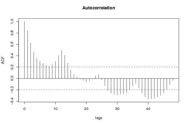
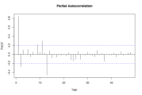
Title produced by software

(Partial) Autocorrelation Function

Date of computation

Thu, 11 Dec 2008 11:26:45 -0700

Cite this page as follows

Statistical Computations at FreeStatistics.org, Office for Research Development and Education, URL https://freestatistics.org/blog/index.php?v=date/2008/Dec/11/t1229020114dtxkbce9keulnt7.htm/, Retrieved Sat, 18 May 2024 08:21:50 +0000

Statistical Computations at FreeStatistics.org, Office for Research Development and Education, URL https://freestatistics.org/blog/index.php?pk=32424, Retrieved Sat, 18 May 2024 08:21:50 +0000

QR Codes:

Paste this QR Code to cite your computation.

Original text written by user:

IsPrivate?

No (this computation is public)

User-defined keywords

Estimated Impact

148

Family? (F = Feedback message, R = changed R code, M = changed R Module, P = changed Parameters, D = changed Data)

-       [(Partial) Autocorrelation Function] [opgave 6 bis oefe...] [2008-12-11 18:26:45] [8318384c9bdcc6ef9a73ee2012b12620] [Current]

Feedback Forum

Post a new message

Dataseries X:

Download CSV

Histogram

Boxplots

Summary of computational transaction
Raw Input	view raw input (R code)
Raw Output	view raw output of R engine
Computing time	1 seconds
R Server	'Gwilym Jenkins' @ 72.249.127.135

\begin{tabular}{lllllllll}
\hline
Summary of computational transaction \tabularnewline
Raw Input & view raw input (R code)  \tabularnewline
Raw Output & view raw output of R engine  \tabularnewline
Computing time & 1 seconds \tabularnewline
R Server & 'Gwilym Jenkins' @ 72.249.127.135 \tabularnewline
\hline
\end{tabular}
%Source: https://freestatistics.org/blog/index.php?pk=32424&T=0

[TABLE]
[ROW][C]Summary of computational transaction[/C][/ROW]
[ROW][C]Raw Input[/C][C]view raw input (R code) [/C][/ROW]
[ROW][C]Raw Output[/C][C]view raw output of R engine [/C][/ROW]
[ROW][C]Computing time[/C][C]1 seconds[/C][/ROW]
[ROW][C]R Server[/C][C]'Gwilym Jenkins' @ 72.249.127.135[/C][/ROW]
[/TABLE]
Source: https://freestatistics.org/blog/index.php?pk=32424&T=0

Globally Unique Identifier (entire table): ba.freestatistics.org/blog/index.php?pk=32424&T=0

As an alternative you can also use a QR Code:

The GUIDs for individual cells are displayed in the table below:

Summary of computational transaction
Raw Input	view raw input (R code)
Raw Output	view raw output of R engine
Computing time	1 seconds
R Server	'Gwilym Jenkins' @ 72.249.127.135

Autocorrelation Function
Time lag k	ACF(k)	T-STAT	P-value
1	0.840163	8.2319	0
2	0.624213	6.116	0
3	0.464102	4.5473	8e-06
4	0.355112	3.4794	0.000379
5	0.306148	2.9996	0.001722
6	0.266516	2.6113	0.005233
7	0.235495	2.3074	0.011591
8	0.21285	2.0855	0.019839
9	0.244213	2.3928	0.009333
10	0.301824	2.9573	0.001953
11	0.404442	3.9627	7.1e-05
12	0.496651	4.8662	2e-06
13	0.407024	3.988	6.5e-05
14	0.268491	2.6307	0.004964
15	0.151095	1.4804	0.071017
16	0.07012	0.687	0.246859
17	0.027527	0.2697	0.39398
18	-0.009045	-0.0886	0.464784
19	-0.03997	-0.3916	0.348102
20	-0.062453	-0.6119	0.271022
21	-0.044194	-0.433	0.33299
22	-0.005326	-0.0522	0.479246
23	0.047166	0.4621	0.322515
24	0.071131	0.6969	0.243762
25	-0.022814	-0.2235	0.411797
26	-0.125603	-1.2307	0.11073
27	-0.210626	-2.0637	0.020872
28	-0.262675	-2.5737	0.005796
29	-0.281153	-2.7547	0.003514
30	-0.286366	-2.8058	0.003039
31	-0.280578	-2.7491	0.00357
32	-0.275005	-2.6945	0.004161
33	-0.251269	-2.4619	0.007802
34	-0.199583	-1.9555	0.026716
35	-0.129134	-1.2652	0.104422
36	-0.089151	-0.8735	0.192286
37	-0.162357	-1.5908	0.057475
38	-0.254177	-2.4904	0.007239
39	-0.323979	-3.1743	0.001009
40	-0.36041	-3.5313	0.000319
41	-0.356014	-3.4882	0.000368
42	-0.345718	-3.3873	0.000512
43	-0.326599	-3.2	0.000932
44	-0.294089	-2.8815	0.002442
45	-0.25152	-2.4644	0.007751
46	-0.192562	-1.8867	0.03111
47	-0.112203	-1.0994	0.13718
48	-0.039687	-0.3889	0.349123

\begin{tabular}{lllllllll}
\hline
Autocorrelation Function \tabularnewline
Time lag k & ACF(k) & T-STAT & P-value \tabularnewline
1 & 0.840163 & 8.2319 & 0 \tabularnewline
2 & 0.624213 & 6.116 & 0 \tabularnewline
3 & 0.464102 & 4.5473 & 8e-06 \tabularnewline
4 & 0.355112 & 3.4794 & 0.000379 \tabularnewline
5 & 0.306148 & 2.9996 & 0.001722 \tabularnewline
6 & 0.266516 & 2.6113 & 0.005233 \tabularnewline
7 & 0.235495 & 2.3074 & 0.011591 \tabularnewline
8 & 0.21285 & 2.0855 & 0.019839 \tabularnewline
9 & 0.244213 & 2.3928 & 0.009333 \tabularnewline
10 & 0.301824 & 2.9573 & 0.001953 \tabularnewline
11 & 0.404442 & 3.9627 & 7.1e-05 \tabularnewline
12 & 0.496651 & 4.8662 & 2e-06 \tabularnewline
13 & 0.407024 & 3.988 & 6.5e-05 \tabularnewline
14 & 0.268491 & 2.6307 & 0.004964 \tabularnewline
15 & 0.151095 & 1.4804 & 0.071017 \tabularnewline
16 & 0.07012 & 0.687 & 0.246859 \tabularnewline
17 & 0.027527 & 0.2697 & 0.39398 \tabularnewline
18 & -0.009045 & -0.0886 & 0.464784 \tabularnewline
19 & -0.03997 & -0.3916 & 0.348102 \tabularnewline
20 & -0.062453 & -0.6119 & 0.271022 \tabularnewline
21 & -0.044194 & -0.433 & 0.33299 \tabularnewline
22 & -0.005326 & -0.0522 & 0.479246 \tabularnewline
23 & 0.047166 & 0.4621 & 0.322515 \tabularnewline
24 & 0.071131 & 0.6969 & 0.243762 \tabularnewline
25 & -0.022814 & -0.2235 & 0.411797 \tabularnewline
26 & -0.125603 & -1.2307 & 0.11073 \tabularnewline
27 & -0.210626 & -2.0637 & 0.020872 \tabularnewline
28 & -0.262675 & -2.5737 & 0.005796 \tabularnewline
29 & -0.281153 & -2.7547 & 0.003514 \tabularnewline
30 & -0.286366 & -2.8058 & 0.003039 \tabularnewline
31 & -0.280578 & -2.7491 & 0.00357 \tabularnewline
32 & -0.275005 & -2.6945 & 0.004161 \tabularnewline
33 & -0.251269 & -2.4619 & 0.007802 \tabularnewline
34 & -0.199583 & -1.9555 & 0.026716 \tabularnewline
35 & -0.129134 & -1.2652 & 0.104422 \tabularnewline
36 & -0.089151 & -0.8735 & 0.192286 \tabularnewline
37 & -0.162357 & -1.5908 & 0.057475 \tabularnewline
38 & -0.254177 & -2.4904 & 0.007239 \tabularnewline
39 & -0.323979 & -3.1743 & 0.001009 \tabularnewline
40 & -0.36041 & -3.5313 & 0.000319 \tabularnewline
41 & -0.356014 & -3.4882 & 0.000368 \tabularnewline
42 & -0.345718 & -3.3873 & 0.000512 \tabularnewline
43 & -0.326599 & -3.2 & 0.000932 \tabularnewline
44 & -0.294089 & -2.8815 & 0.002442 \tabularnewline
45 & -0.25152 & -2.4644 & 0.007751 \tabularnewline
46 & -0.192562 & -1.8867 & 0.03111 \tabularnewline
47 & -0.112203 & -1.0994 & 0.13718 \tabularnewline
48 & -0.039687 & -0.3889 & 0.349123 \tabularnewline
\hline
\end{tabular}
%Source: https://freestatistics.org/blog/index.php?pk=32424&T=1

[TABLE]
[ROW][C]Autocorrelation Function[/C][/ROW]
[ROW][C]Time lag k[/C][C]ACF(k)[/C][C]T-STAT[/C][C]P-value[/C][/ROW]
[ROW][C]1[/C][C]0.840163[/C][C]8.2319[/C][C]0[/C][/ROW]
[ROW][C]2[/C][C]0.624213[/C][C]6.116[/C][C]0[/C][/ROW]
[ROW][C]3[/C][C]0.464102[/C][C]4.5473[/C][C]8e-06[/C][/ROW]
[ROW][C]4[/C][C]0.355112[/C][C]3.4794[/C][C]0.000379[/C][/ROW]
[ROW][C]5[/C][C]0.306148[/C][C]2.9996[/C][C]0.001722[/C][/ROW]
[ROW][C]6[/C][C]0.266516[/C][C]2.6113[/C][C]0.005233[/C][/ROW]
[ROW][C]7[/C][C]0.235495[/C][C]2.3074[/C][C]0.011591[/C][/ROW]
[ROW][C]8[/C][C]0.21285[/C][C]2.0855[/C][C]0.019839[/C][/ROW]
[ROW][C]9[/C][C]0.244213[/C][C]2.3928[/C][C]0.009333[/C][/ROW]
[ROW][C]10[/C][C]0.301824[/C][C]2.9573[/C][C]0.001953[/C][/ROW]
[ROW][C]11[/C][C]0.404442[/C][C]3.9627[/C][C]7.1e-05[/C][/ROW]
[ROW][C]12[/C][C]0.496651[/C][C]4.8662[/C][C]2e-06[/C][/ROW]
[ROW][C]13[/C][C]0.407024[/C][C]3.988[/C][C]6.5e-05[/C][/ROW]
[ROW][C]14[/C][C]0.268491[/C][C]2.6307[/C][C]0.004964[/C][/ROW]
[ROW][C]15[/C][C]0.151095[/C][C]1.4804[/C][C]0.071017[/C][/ROW]
[ROW][C]16[/C][C]0.07012[/C][C]0.687[/C][C]0.246859[/C][/ROW]
[ROW][C]17[/C][C]0.027527[/C][C]0.2697[/C][C]0.39398[/C][/ROW]
[ROW][C]18[/C][C]-0.009045[/C][C]-0.0886[/C][C]0.464784[/C][/ROW]
[ROW][C]19[/C][C]-0.03997[/C][C]-0.3916[/C][C]0.348102[/C][/ROW]
[ROW][C]20[/C][C]-0.062453[/C][C]-0.6119[/C][C]0.271022[/C][/ROW]
[ROW][C]21[/C][C]-0.044194[/C][C]-0.433[/C][C]0.33299[/C][/ROW]
[ROW][C]22[/C][C]-0.005326[/C][C]-0.0522[/C][C]0.479246[/C][/ROW]
[ROW][C]23[/C][C]0.047166[/C][C]0.4621[/C][C]0.322515[/C][/ROW]
[ROW][C]24[/C][C]0.071131[/C][C]0.6969[/C][C]0.243762[/C][/ROW]
[ROW][C]25[/C][C]-0.022814[/C][C]-0.2235[/C][C]0.411797[/C][/ROW]
[ROW][C]26[/C][C]-0.125603[/C][C]-1.2307[/C][C]0.11073[/C][/ROW]
[ROW][C]27[/C][C]-0.210626[/C][C]-2.0637[/C][C]0.020872[/C][/ROW]
[ROW][C]28[/C][C]-0.262675[/C][C]-2.5737[/C][C]0.005796[/C][/ROW]
[ROW][C]29[/C][C]-0.281153[/C][C]-2.7547[/C][C]0.003514[/C][/ROW]
[ROW][C]30[/C][C]-0.286366[/C][C]-2.8058[/C][C]0.003039[/C][/ROW]
[ROW][C]31[/C][C]-0.280578[/C][C]-2.7491[/C][C]0.00357[/C][/ROW]
[ROW][C]32[/C][C]-0.275005[/C][C]-2.6945[/C][C]0.004161[/C][/ROW]
[ROW][C]33[/C][C]-0.251269[/C][C]-2.4619[/C][C]0.007802[/C][/ROW]
[ROW][C]34[/C][C]-0.199583[/C][C]-1.9555[/C][C]0.026716[/C][/ROW]
[ROW][C]35[/C][C]-0.129134[/C][C]-1.2652[/C][C]0.104422[/C][/ROW]
[ROW][C]36[/C][C]-0.089151[/C][C]-0.8735[/C][C]0.192286[/C][/ROW]
[ROW][C]37[/C][C]-0.162357[/C][C]-1.5908[/C][C]0.057475[/C][/ROW]
[ROW][C]38[/C][C]-0.254177[/C][C]-2.4904[/C][C]0.007239[/C][/ROW]
[ROW][C]39[/C][C]-0.323979[/C][C]-3.1743[/C][C]0.001009[/C][/ROW]
[ROW][C]40[/C][C]-0.36041[/C][C]-3.5313[/C][C]0.000319[/C][/ROW]
[ROW][C]41[/C][C]-0.356014[/C][C]-3.4882[/C][C]0.000368[/C][/ROW]
[ROW][C]42[/C][C]-0.345718[/C][C]-3.3873[/C][C]0.000512[/C][/ROW]
[ROW][C]43[/C][C]-0.326599[/C][C]-3.2[/C][C]0.000932[/C][/ROW]
[ROW][C]44[/C][C]-0.294089[/C][C]-2.8815[/C][C]0.002442[/C][/ROW]
[ROW][C]45[/C][C]-0.25152[/C][C]-2.4644[/C][C]0.007751[/C][/ROW]
[ROW][C]46[/C][C]-0.192562[/C][C]-1.8867[/C][C]0.03111[/C][/ROW]
[ROW][C]47[/C][C]-0.112203[/C][C]-1.0994[/C][C]0.13718[/C][/ROW]
[ROW][C]48[/C][C]-0.039687[/C][C]-0.3889[/C][C]0.349123[/C][/ROW]
[/TABLE]
Source: https://freestatistics.org/blog/index.php?pk=32424&T=1

Globally Unique Identifier (entire table): ba.freestatistics.org/blog/index.php?pk=32424&T=1

As an alternative you can also use a QR Code:

The GUIDs for individual cells are displayed in the table below:

Autocorrelation Function
Time lag k	ACF(k)	T-STAT	P-value
1	0.840163	8.2319	0
2	0.624213	6.116	0
3	0.464102	4.5473	8e-06
4	0.355112	3.4794	0.000379
5	0.306148	2.9996	0.001722
6	0.266516	2.6113	0.005233
7	0.235495	2.3074	0.011591
8	0.21285	2.0855	0.019839
9	0.244213	2.3928	0.009333
10	0.301824	2.9573	0.001953
11	0.404442	3.9627	7.1e-05
12	0.496651	4.8662	2e-06
13	0.407024	3.988	6.5e-05
14	0.268491	2.6307	0.004964
15	0.151095	1.4804	0.071017
16	0.07012	0.687	0.246859
17	0.027527	0.2697	0.39398
18	-0.009045	-0.0886	0.464784
19	-0.03997	-0.3916	0.348102
20	-0.062453	-0.6119	0.271022
21	-0.044194	-0.433	0.33299
22	-0.005326	-0.0522	0.479246
23	0.047166	0.4621	0.322515
24	0.071131	0.6969	0.243762
25	-0.022814	-0.2235	0.411797
26	-0.125603	-1.2307	0.11073
27	-0.210626	-2.0637	0.020872
28	-0.262675	-2.5737	0.005796
29	-0.281153	-2.7547	0.003514
30	-0.286366	-2.8058	0.003039
31	-0.280578	-2.7491	0.00357
32	-0.275005	-2.6945	0.004161
33	-0.251269	-2.4619	0.007802
34	-0.199583	-1.9555	0.026716
35	-0.129134	-1.2652	0.104422
36	-0.089151	-0.8735	0.192286
37	-0.162357	-1.5908	0.057475
38	-0.254177	-2.4904	0.007239
39	-0.323979	-3.1743	0.001009
40	-0.36041	-3.5313	0.000319
41	-0.356014	-3.4882	0.000368
42	-0.345718	-3.3873	0.000512
43	-0.326599	-3.2	0.000932
44	-0.294089	-2.8815	0.002442
45	-0.25152	-2.4644	0.007751
46	-0.192562	-1.8867	0.03111
47	-0.112203	-1.0994	0.13718
48	-0.039687	-0.3889	0.349123

Partial Autocorrelation Function
Time lag k	PACF(k)	T-STAT	P-value
1	0.840163	8.2319	0
2	-0.277641	-2.7203	0.003872
3	0.100641	0.9861	0.163288
4	0.000562	0.0055	0.497809
5	0.115525	1.1319	0.130247
6	-0.055542	-0.5442	0.293784
7	0.057477	0.5632	0.287321
8	0.005987	0.0587	0.476671
9	0.217467	2.1307	0.017833
10	0.049285	0.4829	0.315134
11	0.300459	2.9439	0.002032
12	0.035349	0.3463	0.364919
13	-0.458852	-4.4958	1e-05
14	0.081517	0.7987	0.213219
15	-0.082066	-0.8041	0.211668
16	-0.010199	-0.0999	0.460304
17	-0.062592	-0.6133	0.270572
18	-0.014811	-0.1451	0.44246
19	-0.018715	-0.1834	0.427449
20	0.005282	0.0517	0.479418
21	-0.030608	-0.2999	0.382452
22	0.042485	0.4163	0.339071
23	-0.125354	-1.2282	0.111185
24	-0.145596	-1.4265	0.078477
25	-0.110355	-1.0812	0.141147
26	0.068589	0.672	0.251587
27	-0.10932	-1.0711	0.143401
28	0.006995	0.0685	0.472749
29	-0.021869	-0.2143	0.415396
30	0.051223	0.5019	0.308451
31	-0.015666	-0.1535	0.439164
32	-0.0261	-0.2557	0.399353
33	-0.055763	-0.5464	0.293043
34	0.091276	0.8943	0.186693
35	-0.013115	-0.1285	0.44901
36	0.026081	0.2555	0.399428
37	-0.154171	-1.5106	0.067093
38	-0.008742	-0.0857	0.465959
39	-0.012502	-0.1225	0.451381
40	-0.013554	-0.1328	0.447315
41	0.031754	0.3111	0.378189
42	-0.063376	-0.621	0.268049
43	-0.013799	-0.1352	0.446367
44	0.063436	0.6215	0.267857
45	-0.02122	-0.2079	0.417869
46	0.004051	0.0397	0.484209
47	0.035061	0.3435	0.365975
48	0.049537	0.4854	0.314264

\begin{tabular}{lllllllll}
\hline
Partial Autocorrelation Function \tabularnewline
Time lag k & PACF(k) & T-STAT & P-value \tabularnewline
1 & 0.840163 & 8.2319 & 0 \tabularnewline
2 & -0.277641 & -2.7203 & 0.003872 \tabularnewline
3 & 0.100641 & 0.9861 & 0.163288 \tabularnewline
4 & 0.000562 & 0.0055 & 0.497809 \tabularnewline
5 & 0.115525 & 1.1319 & 0.130247 \tabularnewline
6 & -0.055542 & -0.5442 & 0.293784 \tabularnewline
7 & 0.057477 & 0.5632 & 0.287321 \tabularnewline
8 & 0.005987 & 0.0587 & 0.476671 \tabularnewline
9 & 0.217467 & 2.1307 & 0.017833 \tabularnewline
10 & 0.049285 & 0.4829 & 0.315134 \tabularnewline
11 & 0.300459 & 2.9439 & 0.002032 \tabularnewline
12 & 0.035349 & 0.3463 & 0.364919 \tabularnewline
13 & -0.458852 & -4.4958 & 1e-05 \tabularnewline
14 & 0.081517 & 0.7987 & 0.213219 \tabularnewline
15 & -0.082066 & -0.8041 & 0.211668 \tabularnewline
16 & -0.010199 & -0.0999 & 0.460304 \tabularnewline
17 & -0.062592 & -0.6133 & 0.270572 \tabularnewline
18 & -0.014811 & -0.1451 & 0.44246 \tabularnewline
19 & -0.018715 & -0.1834 & 0.427449 \tabularnewline
20 & 0.005282 & 0.0517 & 0.479418 \tabularnewline
21 & -0.030608 & -0.2999 & 0.382452 \tabularnewline
22 & 0.042485 & 0.4163 & 0.339071 \tabularnewline
23 & -0.125354 & -1.2282 & 0.111185 \tabularnewline
24 & -0.145596 & -1.4265 & 0.078477 \tabularnewline
25 & -0.110355 & -1.0812 & 0.141147 \tabularnewline
26 & 0.068589 & 0.672 & 0.251587 \tabularnewline
27 & -0.10932 & -1.0711 & 0.143401 \tabularnewline
28 & 0.006995 & 0.0685 & 0.472749 \tabularnewline
29 & -0.021869 & -0.2143 & 0.415396 \tabularnewline
30 & 0.051223 & 0.5019 & 0.308451 \tabularnewline
31 & -0.015666 & -0.1535 & 0.439164 \tabularnewline
32 & -0.0261 & -0.2557 & 0.399353 \tabularnewline
33 & -0.055763 & -0.5464 & 0.293043 \tabularnewline
34 & 0.091276 & 0.8943 & 0.186693 \tabularnewline
35 & -0.013115 & -0.1285 & 0.44901 \tabularnewline
36 & 0.026081 & 0.2555 & 0.399428 \tabularnewline
37 & -0.154171 & -1.5106 & 0.067093 \tabularnewline
38 & -0.008742 & -0.0857 & 0.465959 \tabularnewline
39 & -0.012502 & -0.1225 & 0.451381 \tabularnewline
40 & -0.013554 & -0.1328 & 0.447315 \tabularnewline
41 & 0.031754 & 0.3111 & 0.378189 \tabularnewline
42 & -0.063376 & -0.621 & 0.268049 \tabularnewline
43 & -0.013799 & -0.1352 & 0.446367 \tabularnewline
44 & 0.063436 & 0.6215 & 0.267857 \tabularnewline
45 & -0.02122 & -0.2079 & 0.417869 \tabularnewline
46 & 0.004051 & 0.0397 & 0.484209 \tabularnewline
47 & 0.035061 & 0.3435 & 0.365975 \tabularnewline
48 & 0.049537 & 0.4854 & 0.314264 \tabularnewline
\hline
\end{tabular}
%Source: https://freestatistics.org/blog/index.php?pk=32424&T=2

[TABLE]
[ROW][C]Partial Autocorrelation Function[/C][/ROW]
[ROW][C]Time lag k[/C][C]PACF(k)[/C][C]T-STAT[/C][C]P-value[/C][/ROW]
[ROW][C]1[/C][C]0.840163[/C][C]8.2319[/C][C]0[/C][/ROW]
[ROW][C]2[/C][C]-0.277641[/C][C]-2.7203[/C][C]0.003872[/C][/ROW]
[ROW][C]3[/C][C]0.100641[/C][C]0.9861[/C][C]0.163288[/C][/ROW]
[ROW][C]4[/C][C]0.000562[/C][C]0.0055[/C][C]0.497809[/C][/ROW]
[ROW][C]5[/C][C]0.115525[/C][C]1.1319[/C][C]0.130247[/C][/ROW]
[ROW][C]6[/C][C]-0.055542[/C][C]-0.5442[/C][C]0.293784[/C][/ROW]
[ROW][C]7[/C][C]0.057477[/C][C]0.5632[/C][C]0.287321[/C][/ROW]
[ROW][C]8[/C][C]0.005987[/C][C]0.0587[/C][C]0.476671[/C][/ROW]
[ROW][C]9[/C][C]0.217467[/C][C]2.1307[/C][C]0.017833[/C][/ROW]
[ROW][C]10[/C][C]0.049285[/C][C]0.4829[/C][C]0.315134[/C][/ROW]
[ROW][C]11[/C][C]0.300459[/C][C]2.9439[/C][C]0.002032[/C][/ROW]
[ROW][C]12[/C][C]0.035349[/C][C]0.3463[/C][C]0.364919[/C][/ROW]
[ROW][C]13[/C][C]-0.458852[/C][C]-4.4958[/C][C]1e-05[/C][/ROW]
[ROW][C]14[/C][C]0.081517[/C][C]0.7987[/C][C]0.213219[/C][/ROW]
[ROW][C]15[/C][C]-0.082066[/C][C]-0.8041[/C][C]0.211668[/C][/ROW]
[ROW][C]16[/C][C]-0.010199[/C][C]-0.0999[/C][C]0.460304[/C][/ROW]
[ROW][C]17[/C][C]-0.062592[/C][C]-0.6133[/C][C]0.270572[/C][/ROW]
[ROW][C]18[/C][C]-0.014811[/C][C]-0.1451[/C][C]0.44246[/C][/ROW]
[ROW][C]19[/C][C]-0.018715[/C][C]-0.1834[/C][C]0.427449[/C][/ROW]
[ROW][C]20[/C][C]0.005282[/C][C]0.0517[/C][C]0.479418[/C][/ROW]
[ROW][C]21[/C][C]-0.030608[/C][C]-0.2999[/C][C]0.382452[/C][/ROW]
[ROW][C]22[/C][C]0.042485[/C][C]0.4163[/C][C]0.339071[/C][/ROW]
[ROW][C]23[/C][C]-0.125354[/C][C]-1.2282[/C][C]0.111185[/C][/ROW]
[ROW][C]24[/C][C]-0.145596[/C][C]-1.4265[/C][C]0.078477[/C][/ROW]
[ROW][C]25[/C][C]-0.110355[/C][C]-1.0812[/C][C]0.141147[/C][/ROW]
[ROW][C]26[/C][C]0.068589[/C][C]0.672[/C][C]0.251587[/C][/ROW]
[ROW][C]27[/C][C]-0.10932[/C][C]-1.0711[/C][C]0.143401[/C][/ROW]
[ROW][C]28[/C][C]0.006995[/C][C]0.0685[/C][C]0.472749[/C][/ROW]
[ROW][C]29[/C][C]-0.021869[/C][C]-0.2143[/C][C]0.415396[/C][/ROW]
[ROW][C]30[/C][C]0.051223[/C][C]0.5019[/C][C]0.308451[/C][/ROW]
[ROW][C]31[/C][C]-0.015666[/C][C]-0.1535[/C][C]0.439164[/C][/ROW]
[ROW][C]32[/C][C]-0.0261[/C][C]-0.2557[/C][C]0.399353[/C][/ROW]
[ROW][C]33[/C][C]-0.055763[/C][C]-0.5464[/C][C]0.293043[/C][/ROW]
[ROW][C]34[/C][C]0.091276[/C][C]0.8943[/C][C]0.186693[/C][/ROW]
[ROW][C]35[/C][C]-0.013115[/C][C]-0.1285[/C][C]0.44901[/C][/ROW]
[ROW][C]36[/C][C]0.026081[/C][C]0.2555[/C][C]0.399428[/C][/ROW]
[ROW][C]37[/C][C]-0.154171[/C][C]-1.5106[/C][C]0.067093[/C][/ROW]
[ROW][C]38[/C][C]-0.008742[/C][C]-0.0857[/C][C]0.465959[/C][/ROW]
[ROW][C]39[/C][C]-0.012502[/C][C]-0.1225[/C][C]0.451381[/C][/ROW]
[ROW][C]40[/C][C]-0.013554[/C][C]-0.1328[/C][C]0.447315[/C][/ROW]
[ROW][C]41[/C][C]0.031754[/C][C]0.3111[/C][C]0.378189[/C][/ROW]
[ROW][C]42[/C][C]-0.063376[/C][C]-0.621[/C][C]0.268049[/C][/ROW]
[ROW][C]43[/C][C]-0.013799[/C][C]-0.1352[/C][C]0.446367[/C][/ROW]
[ROW][C]44[/C][C]0.063436[/C][C]0.6215[/C][C]0.267857[/C][/ROW]
[ROW][C]45[/C][C]-0.02122[/C][C]-0.2079[/C][C]0.417869[/C][/ROW]
[ROW][C]46[/C][C]0.004051[/C][C]0.0397[/C][C]0.484209[/C][/ROW]
[ROW][C]47[/C][C]0.035061[/C][C]0.3435[/C][C]0.365975[/C][/ROW]
[ROW][C]48[/C][C]0.049537[/C][C]0.4854[/C][C]0.314264[/C][/ROW]
[/TABLE]
Source: https://freestatistics.org/blog/index.php?pk=32424&T=2

Globally Unique Identifier (entire table): ba.freestatistics.org/blog/index.php?pk=32424&T=2

As an alternative you can also use a QR Code:

The GUIDs for individual cells are displayed in the table below:

Partial Autocorrelation Function
Time lag k	PACF(k)	T-STAT	P-value
1	0.840163	8.2319	0
2	-0.277641	-2.7203	0.003872
3	0.100641	0.9861	0.163288
4	0.000562	0.0055	0.497809
5	0.115525	1.1319	0.130247
6	-0.055542	-0.5442	0.293784
7	0.057477	0.5632	0.287321
8	0.005987	0.0587	0.476671
9	0.217467	2.1307	0.017833
10	0.049285	0.4829	0.315134
11	0.300459	2.9439	0.002032
12	0.035349	0.3463	0.364919
13	-0.458852	-4.4958	1e-05
14	0.081517	0.7987	0.213219
15	-0.082066	-0.8041	0.211668
16	-0.010199	-0.0999	0.460304
17	-0.062592	-0.6133	0.270572
18	-0.014811	-0.1451	0.44246
19	-0.018715	-0.1834	0.427449
20	0.005282	0.0517	0.479418
21	-0.030608	-0.2999	0.382452
22	0.042485	0.4163	0.339071
23	-0.125354	-1.2282	0.111185
24	-0.145596	-1.4265	0.078477
25	-0.110355	-1.0812	0.141147
26	0.068589	0.672	0.251587
27	-0.10932	-1.0711	0.143401
28	0.006995	0.0685	0.472749
29	-0.021869	-0.2143	0.415396
30	0.051223	0.5019	0.308451
31	-0.015666	-0.1535	0.439164
32	-0.0261	-0.2557	0.399353
33	-0.055763	-0.5464	0.293043
34	0.091276	0.8943	0.186693
35	-0.013115	-0.1285	0.44901
36	0.026081	0.2555	0.399428
37	-0.154171	-1.5106	0.067093
38	-0.008742	-0.0857	0.465959
39	-0.012502	-0.1225	0.451381
40	-0.013554	-0.1328	0.447315
41	0.031754	0.3111	0.378189
42	-0.063376	-0.621	0.268049
43	-0.013799	-0.1352	0.446367
44	0.063436	0.6215	0.267857
45	-0.02122	-0.2079	0.417869
46	0.004051	0.0397	0.484209
47	0.035061	0.3435	0.365975
48	0.049537	0.4854	0.314264

Figure 1

PNG link

Postscript link

PDF link

Figure 2

PNG link

Postscript link

PDF link

Parameters (Session):

par1 = 48 ; par2 = 1 ; par3 = 0 ; par4 = 0 ; par5 = 12 ;

Parameters (R input):

par1 = 48 ; par2 = 1 ; par3 = 0 ; par4 = 0 ; par5 = 12 ;

R code (references can be found in the software module):

if (par1 == 'Default') {
par1 = 10*log10(length(x))
} else {
par1 <- as.numeric(par1)
}
par2 <- as.numeric(par2)
par3 <- as.numeric(par3)
par4 <- as.numeric(par4)
par5 <- as.numeric(par5)
if (par2 == 0) {
x <- log(x)
} else {
x <- (x ^ par2 - 1) / par2
}
if (par3 > 0) x <- diff(x,lag=1,difference=par3)
if (par4 > 0) x <- diff(x,lag=par5,difference=par4)
bitmap(file='pic1.png')
racf <- acf(x,par1,main='Autocorrelation',xlab='lags',ylab='ACF')
dev.off()
bitmap(file='pic2.png')
rpacf <- pacf(x,par1,main='Partial Autocorrelation',xlab='lags',ylab='PACF')
dev.off()
(myacf <- c(racf$acf))
(mypacf <- c(rpacf$acf))
lengthx <- length(x)
sqrtn <- sqrt(lengthx)
load(file='createtable')
a<-table.start()
a<-table.row.start(a)
a<-table.element(a,'Autocorrelation Function',4,TRUE)
a<-table.row.end(a)
a<-table.row.start(a)
a<-table.element(a,'Time lag k',header=TRUE)
a<-table.element(a,hyperlink('basics.htm','ACF(k)','click here for more information about the Autocorrelation Function'),header=TRUE)
a<-table.element(a,'T-STAT',header=TRUE)
a<-table.element(a,'P-value',header=TRUE)
a<-table.row.end(a)
for (i in 2:(par1+1)) {
a<-table.row.start(a)
a<-table.element(a,i-1,header=TRUE)
a<-table.element(a,round(myacf[i],6))
mytstat <- myacf[i]*sqrtn
a<-table.element(a,round(mytstat,4))
a<-table.element(a,round(1-pt(abs(mytstat),lengthx),6))
a<-table.row.end(a)
}
a<-table.end(a)
table.save(a,file='mytable.tab')
a<-table.start()
a<-table.row.start(a)
a<-table.element(a,'Partial Autocorrelation Function',4,TRUE)
a<-table.row.end(a)
a<-table.row.start(a)
a<-table.element(a,'Time lag k',header=TRUE)
a<-table.element(a,hyperlink('basics.htm','PACF(k)','click here for more information about the Partial Autocorrelation Function'),header=TRUE)
a<-table.element(a,'T-STAT',header=TRUE)
a<-table.element(a,'P-value',header=TRUE)
a<-table.row.end(a)
for (i in 1:par1) {
a<-table.row.start(a)
a<-table.element(a,i,header=TRUE)
a<-table.element(a,round(mypacf[i],6))
mytstat <- mypacf[i]*sqrtn
a<-table.element(a,round(mytstat,4))
a<-table.element(a,round(1-pt(abs(mytstat),lengthx),6))
a<-table.row.end(a)
}
a<-table.end(a)
table.save(a,file='mytable1.tab')

Free Statistics

Description of Statistical Computation

Tree of Dependent Computations

Dataset

Tables (Output of Computation)

Figures (Output of Computation)

Input Parameters & R Code