Free Statistics
of Irreproducible Research!
Description of Statistical Computation | |||||||||||||||||||||
|---|---|---|---|---|---|---|---|---|---|---|---|---|---|---|---|---|---|---|---|---|---|
| Author's title | |||||||||||||||||||||
| Author | *The author of this computation has been verified* | ||||||||||||||||||||
| R Software Module | rwasp_meanplot.wasp | ||||||||||||||||||||
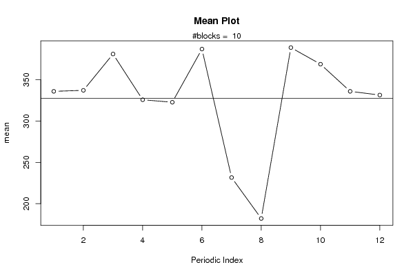
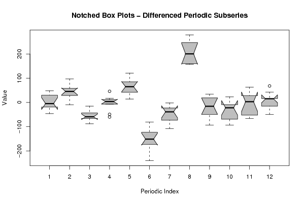
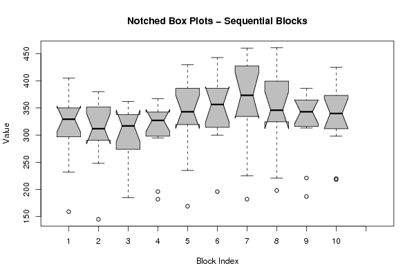
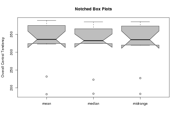
| Title produced by software | Mean Plot | ||||||||||||||||||||
| Date of computation | Sat, 13 Dec 2008 02:58:03 -0700 | ||||||||||||||||||||
| Cite this page as follows | Statistical Computations at FreeStatistics.org, Office for Research Development and Education, URL https://freestatistics.org/blog/index.php?v=date/2008/Dec/13/t1229162370c2mc47bdtsmnuqc.htm/, Retrieved Sat, 18 May 2024 10:07:25 +0000 | ||||||||||||||||||||
| Statistical Computations at FreeStatistics.org, Office for Research Development and Education, URL https://freestatistics.org/blog/index.php?pk=32925, Retrieved Sat, 18 May 2024 10:07:25 +0000 | |||||||||||||||||||||
| QR Codes: | |||||||||||||||||||||
|
| |||||||||||||||||||||
| Original text written by user: | |||||||||||||||||||||
| IsPrivate? | No (this computation is public) | ||||||||||||||||||||
| User-defined keywords | |||||||||||||||||||||
| Estimated Impact | 202 | ||||||||||||||||||||
Tree of Dependent Computations | |||||||||||||||||||||
| Family? (F = Feedback message, R = changed R code, M = changed R Module, P = changed Parameters, D = changed Data) | |||||||||||||||||||||
| - [Mean Plot] [Mean Plot voor he...] [2008-12-13 09:58:03] [6fc58909ffe15c247a4f6748c8841ab4] [Current] - D [Mean Plot] [Mean Plot voor he...] [2008-12-13 10:28:35] [87cabf13a90315c7085b765dcebb7412] | |||||||||||||||||||||
| Feedback Forum | |||||||||||||||||||||
Post a new message | |||||||||||||||||||||
Dataset | |||||||||||||||||||||
| Dataseries X: | |||||||||||||||||||||
293 301 362 330 328 405 232 159 336 361 329 339 290 328 375 294 340 364 248 145 380 305 291 319 334 318 362 296 300 342 215 185 343 333 316 252 320 324 343 295 301 367 196 182 342 361 334 330 345 323 366 323 316 358 235 169 430 409 407 341 326 374 364 349 300 385 304 196 443 414 325 388 356 386 444 387 327 448 225 182 460 411 342 361 377 331 428 340 352 461 221 198 422 329 320 375 364 351 380 319 322 386 221 187 344 342 365 313 356 337 389 326 343 357 220 218 391 425 332 298 | |||||||||||||||||||||
Tables (Output of Computation) | |||||||||||||||||||||
| |||||||||||||||||||||
Figures (Output of Computation) | |||||||||||||||||||||
Input Parameters & R Code | |||||||||||||||||||||
| Parameters (Session): | |||||||||||||||||||||
| par1 = 12 ; | |||||||||||||||||||||
| Parameters (R input): | |||||||||||||||||||||
| par1 = 12 ; | |||||||||||||||||||||
| R code (references can be found in the software module): | |||||||||||||||||||||
par1 <- as.numeric(par1) | |||||||||||||||||||||