Repository of Reproducible Computations

Free Statistics

of Irreproducible Research!

Author's title

Author

*The author of this computation has been verified*

R Software Module

rwasp_autocorrelation.wasp

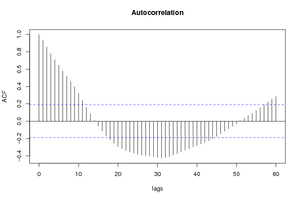
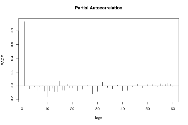
Title produced by software

(Partial) Autocorrelation Function

Date of computation

Sat, 20 Dec 2008 03:51:34 -0700

Cite this page as follows

Statistical Computations at FreeStatistics.org, Office for Research Development and Education, URL https://freestatistics.org/blog/index.php?v=date/2008/Dec/20/t1229770406ibnhydp7k41av59.htm/, Retrieved Sat, 18 May 2024 13:10:40 +0000

Statistical Computations at FreeStatistics.org, Office for Research Development and Education, URL https://freestatistics.org/blog/index.php?pk=35325, Retrieved Sat, 18 May 2024 13:10:40 +0000

QR Codes:

Paste this QR Code to cite your computation.

Original text written by user:

Lambda = 1 d = 0 D = 0 time lags = 60 seasonality = 12

IsPrivate?

No (this computation is public)

User-defined keywords

Estimated Impact

227

Family? (F = Feedback message, R = changed R code, M = changed R Module, P = changed Parameters, D = changed Data)

-       [(Partial) Autocorrelation Function] [Paper - Autocorre...] [2008-12-20 10:51:34] [821c4b3d195be8e737cf8c9dc649d3cf] [Current]
-   P     [(Partial) Autocorrelation Function] [Paper - Autocorre...] [2008-12-20 11:09:54] [3a9fc6d5b5e0e816787b7dbace57e7cd] 
- RMP     [Spectral Analysis] [Paper - spectrale...] [2008-12-20 11:56:10] [3a9fc6d5b5e0e816787b7dbace57e7cd] 
- RMP     [Spectral Analysis] [Paper - spectrale...] [2008-12-20 12:15:58] [3a9fc6d5b5e0e816787b7dbace57e7cd] 
- RMP     [Variance Reduction Matrix] [Paper - Variance ...] [2008-12-20 12:24:21] [3a9fc6d5b5e0e816787b7dbace57e7cd] 
F RMP     [ARIMA Backward Selection] [Paper - ARIMA Bac...] [2008-12-20 13:42:52] [3a9fc6d5b5e0e816787b7dbace57e7cd] 
- RMP     [ARIMA Forecasting] [Paper - ARIMA For...] [2008-12-20 14:29:20] [3a9fc6d5b5e0e816787b7dbace57e7cd] 

Feedback Forum

Post a new message

Dataseries X:

Download CSV

Histogram

Boxplots

Summary of computational transaction
Raw Input	view raw input (R code)
Raw Output	view raw output of R engine
Computing time	3 seconds
R Server	'Herman Ole Andreas Wold' @ 193.190.124.10:1001

\begin{tabular}{lllllllll}
\hline
Summary of computational transaction \tabularnewline
Raw Input & view raw input (R code)  \tabularnewline
Raw Output & view raw output of R engine  \tabularnewline
Computing time & 3 seconds \tabularnewline
R Server & 'Herman Ole Andreas Wold' @ 193.190.124.10:1001 \tabularnewline
\hline
\end{tabular}
%Source: https://freestatistics.org/blog/index.php?pk=35325&T=0

[TABLE]
[ROW][C]Summary of computational transaction[/C][/ROW]
[ROW][C]Raw Input[/C][C]view raw input (R code) [/C][/ROW]
[ROW][C]Raw Output[/C][C]view raw output of R engine [/C][/ROW]
[ROW][C]Computing time[/C][C]3 seconds[/C][/ROW]
[ROW][C]R Server[/C][C]'Herman Ole Andreas Wold' @ 193.190.124.10:1001[/C][/ROW]
[/TABLE]
Source: https://freestatistics.org/blog/index.php?pk=35325&T=0

Globally Unique Identifier (entire table): ba.freestatistics.org/blog/index.php?pk=35325&T=0

As an alternative you can also use a QR Code:

The GUIDs for individual cells are displayed in the table below:

Summary of computational transaction
Raw Input	view raw input (R code)
Raw Output	view raw output of R engine
Computing time	3 seconds
R Server	'Herman Ole Andreas Wold' @ 193.190.124.10:1001

Autocorrelation Function
Time lag k	ACF(k)	T-STAT	P-value
1	0.933218	9.6983	0
2	0.856817	8.9043	0
3	0.779557	8.1014	0
4	0.710569	7.3844	0
5	0.645658	6.7099	0
6	0.578399	6.0109	0
7	0.514864	5.3506	0
8	0.457599	4.7555	3e-06
9	0.396858	4.1243	3.7e-05
10	0.32125	3.3385	0.000578
11	0.240403	2.4983	0.006992
12	0.162739	1.6912	0.046838
13	0.085475	0.8883	0.188181
14	0.0071	0.0738	0.470659
15	-0.054069	-0.5619	0.287672
16	-0.111992	-1.1639	0.123523
17	-0.16668	-1.7322	0.043048
18	-0.212432	-2.2077	0.014692
19	-0.255867	-2.6591	0.004514
20	-0.294175	-3.0572	0.001408
21	-0.315014	-3.2737	0.000713
22	-0.338514	-3.5179	0.000319
23	-0.354485	-3.6839	0.00018
24	-0.368847	-3.8332	0.000106
25	-0.384706	-3.998	5.9e-05
26	-0.393951	-4.0941	4.1e-05
27	-0.394429	-4.099	4e-05
28	-0.400334	-4.1604	3.2e-05
29	-0.409989	-4.2607	2.2e-05
30	-0.42077	-4.3728	1.4e-05
31	-0.428159	-4.4496	1.1e-05
32	-0.421735	-4.3828	1.4e-05
33	-0.408999	-4.2504	2.3e-05
34	-0.393388	-4.0882	4.2e-05
35	-0.375068	-3.8978	8.4e-05
36	-0.354093	-3.6798	0.000183
37	-0.335508	-3.4867	0.000354
38	-0.317378	-3.2983	0.000659
39	-0.296742	-3.0838	0.001297
40	-0.281646	-2.927	0.002087
41	-0.262989	-2.7331	0.003667
42	-0.243124	-2.5266	0.006483
43	-0.224688	-2.335	0.010695
44	-0.202176	-2.1011	0.018981
45	-0.176116	-1.8303	0.034985
46	-0.146531	-1.5228	0.065366
47	-0.116726	-1.2131	0.113878
48	-0.086106	-0.8948	0.186432
49	-0.058835	-0.6114	0.271099
50	-0.027781	-0.2887	0.386678
51	0.005056	0.0525	0.479095
52	0.034459	0.3581	0.36048
53	0.063737	0.6624	0.254571
54	0.092975	0.9662	0.168046
55	0.124142	1.2901	0.099882
56	0.157114	1.6328	0.052715
57	0.190631	1.9811	0.025061
58	0.221925	2.3063	0.011501
59	0.254948	2.6495	0.004636
60	0.285167	2.9635	0.001871

\begin{tabular}{lllllllll}
\hline
Autocorrelation Function \tabularnewline
Time lag k & ACF(k) & T-STAT & P-value \tabularnewline
1 & 0.933218 & 9.6983 & 0 \tabularnewline
2 & 0.856817 & 8.9043 & 0 \tabularnewline
3 & 0.779557 & 8.1014 & 0 \tabularnewline
4 & 0.710569 & 7.3844 & 0 \tabularnewline
5 & 0.645658 & 6.7099 & 0 \tabularnewline
6 & 0.578399 & 6.0109 & 0 \tabularnewline
7 & 0.514864 & 5.3506 & 0 \tabularnewline
8 & 0.457599 & 4.7555 & 3e-06 \tabularnewline
9 & 0.396858 & 4.1243 & 3.7e-05 \tabularnewline
10 & 0.32125 & 3.3385 & 0.000578 \tabularnewline
11 & 0.240403 & 2.4983 & 0.006992 \tabularnewline
12 & 0.162739 & 1.6912 & 0.046838 \tabularnewline
13 & 0.085475 & 0.8883 & 0.188181 \tabularnewline
14 & 0.0071 & 0.0738 & 0.470659 \tabularnewline
15 & -0.054069 & -0.5619 & 0.287672 \tabularnewline
16 & -0.111992 & -1.1639 & 0.123523 \tabularnewline
17 & -0.16668 & -1.7322 & 0.043048 \tabularnewline
18 & -0.212432 & -2.2077 & 0.014692 \tabularnewline
19 & -0.255867 & -2.6591 & 0.004514 \tabularnewline
20 & -0.294175 & -3.0572 & 0.001408 \tabularnewline
21 & -0.315014 & -3.2737 & 0.000713 \tabularnewline
22 & -0.338514 & -3.5179 & 0.000319 \tabularnewline
23 & -0.354485 & -3.6839 & 0.00018 \tabularnewline
24 & -0.368847 & -3.8332 & 0.000106 \tabularnewline
25 & -0.384706 & -3.998 & 5.9e-05 \tabularnewline
26 & -0.393951 & -4.0941 & 4.1e-05 \tabularnewline
27 & -0.394429 & -4.099 & 4e-05 \tabularnewline
28 & -0.400334 & -4.1604 & 3.2e-05 \tabularnewline
29 & -0.409989 & -4.2607 & 2.2e-05 \tabularnewline
30 & -0.42077 & -4.3728 & 1.4e-05 \tabularnewline
31 & -0.428159 & -4.4496 & 1.1e-05 \tabularnewline
32 & -0.421735 & -4.3828 & 1.4e-05 \tabularnewline
33 & -0.408999 & -4.2504 & 2.3e-05 \tabularnewline
34 & -0.393388 & -4.0882 & 4.2e-05 \tabularnewline
35 & -0.375068 & -3.8978 & 8.4e-05 \tabularnewline
36 & -0.354093 & -3.6798 & 0.000183 \tabularnewline
37 & -0.335508 & -3.4867 & 0.000354 \tabularnewline
38 & -0.317378 & -3.2983 & 0.000659 \tabularnewline
39 & -0.296742 & -3.0838 & 0.001297 \tabularnewline
40 & -0.281646 & -2.927 & 0.002087 \tabularnewline
41 & -0.262989 & -2.7331 & 0.003667 \tabularnewline
42 & -0.243124 & -2.5266 & 0.006483 \tabularnewline
43 & -0.224688 & -2.335 & 0.010695 \tabularnewline
44 & -0.202176 & -2.1011 & 0.018981 \tabularnewline
45 & -0.176116 & -1.8303 & 0.034985 \tabularnewline
46 & -0.146531 & -1.5228 & 0.065366 \tabularnewline
47 & -0.116726 & -1.2131 & 0.113878 \tabularnewline
48 & -0.086106 & -0.8948 & 0.186432 \tabularnewline
49 & -0.058835 & -0.6114 & 0.271099 \tabularnewline
50 & -0.027781 & -0.2887 & 0.386678 \tabularnewline
51 & 0.005056 & 0.0525 & 0.479095 \tabularnewline
52 & 0.034459 & 0.3581 & 0.36048 \tabularnewline
53 & 0.063737 & 0.6624 & 0.254571 \tabularnewline
54 & 0.092975 & 0.9662 & 0.168046 \tabularnewline
55 & 0.124142 & 1.2901 & 0.099882 \tabularnewline
56 & 0.157114 & 1.6328 & 0.052715 \tabularnewline
57 & 0.190631 & 1.9811 & 0.025061 \tabularnewline
58 & 0.221925 & 2.3063 & 0.011501 \tabularnewline
59 & 0.254948 & 2.6495 & 0.004636 \tabularnewline
60 & 0.285167 & 2.9635 & 0.001871 \tabularnewline
\hline
\end{tabular}
%Source: https://freestatistics.org/blog/index.php?pk=35325&T=1

[TABLE]
[ROW][C]Autocorrelation Function[/C][/ROW]
[ROW][C]Time lag k[/C][C]ACF(k)[/C][C]T-STAT[/C][C]P-value[/C][/ROW]
[ROW][C]1[/C][C]0.933218[/C][C]9.6983[/C][C]0[/C][/ROW]
[ROW][C]2[/C][C]0.856817[/C][C]8.9043[/C][C]0[/C][/ROW]
[ROW][C]3[/C][C]0.779557[/C][C]8.1014[/C][C]0[/C][/ROW]
[ROW][C]4[/C][C]0.710569[/C][C]7.3844[/C][C]0[/C][/ROW]
[ROW][C]5[/C][C]0.645658[/C][C]6.7099[/C][C]0[/C][/ROW]
[ROW][C]6[/C][C]0.578399[/C][C]6.0109[/C][C]0[/C][/ROW]
[ROW][C]7[/C][C]0.514864[/C][C]5.3506[/C][C]0[/C][/ROW]
[ROW][C]8[/C][C]0.457599[/C][C]4.7555[/C][C]3e-06[/C][/ROW]
[ROW][C]9[/C][C]0.396858[/C][C]4.1243[/C][C]3.7e-05[/C][/ROW]
[ROW][C]10[/C][C]0.32125[/C][C]3.3385[/C][C]0.000578[/C][/ROW]
[ROW][C]11[/C][C]0.240403[/C][C]2.4983[/C][C]0.006992[/C][/ROW]
[ROW][C]12[/C][C]0.162739[/C][C]1.6912[/C][C]0.046838[/C][/ROW]
[ROW][C]13[/C][C]0.085475[/C][C]0.8883[/C][C]0.188181[/C][/ROW]
[ROW][C]14[/C][C]0.0071[/C][C]0.0738[/C][C]0.470659[/C][/ROW]
[ROW][C]15[/C][C]-0.054069[/C][C]-0.5619[/C][C]0.287672[/C][/ROW]
[ROW][C]16[/C][C]-0.111992[/C][C]-1.1639[/C][C]0.123523[/C][/ROW]
[ROW][C]17[/C][C]-0.16668[/C][C]-1.7322[/C][C]0.043048[/C][/ROW]
[ROW][C]18[/C][C]-0.212432[/C][C]-2.2077[/C][C]0.014692[/C][/ROW]
[ROW][C]19[/C][C]-0.255867[/C][C]-2.6591[/C][C]0.004514[/C][/ROW]
[ROW][C]20[/C][C]-0.294175[/C][C]-3.0572[/C][C]0.001408[/C][/ROW]
[ROW][C]21[/C][C]-0.315014[/C][C]-3.2737[/C][C]0.000713[/C][/ROW]
[ROW][C]22[/C][C]-0.338514[/C][C]-3.5179[/C][C]0.000319[/C][/ROW]
[ROW][C]23[/C][C]-0.354485[/C][C]-3.6839[/C][C]0.00018[/C][/ROW]
[ROW][C]24[/C][C]-0.368847[/C][C]-3.8332[/C][C]0.000106[/C][/ROW]
[ROW][C]25[/C][C]-0.384706[/C][C]-3.998[/C][C]5.9e-05[/C][/ROW]
[ROW][C]26[/C][C]-0.393951[/C][C]-4.0941[/C][C]4.1e-05[/C][/ROW]
[ROW][C]27[/C][C]-0.394429[/C][C]-4.099[/C][C]4e-05[/C][/ROW]
[ROW][C]28[/C][C]-0.400334[/C][C]-4.1604[/C][C]3.2e-05[/C][/ROW]
[ROW][C]29[/C][C]-0.409989[/C][C]-4.2607[/C][C]2.2e-05[/C][/ROW]
[ROW][C]30[/C][C]-0.42077[/C][C]-4.3728[/C][C]1.4e-05[/C][/ROW]
[ROW][C]31[/C][C]-0.428159[/C][C]-4.4496[/C][C]1.1e-05[/C][/ROW]
[ROW][C]32[/C][C]-0.421735[/C][C]-4.3828[/C][C]1.4e-05[/C][/ROW]
[ROW][C]33[/C][C]-0.408999[/C][C]-4.2504[/C][C]2.3e-05[/C][/ROW]
[ROW][C]34[/C][C]-0.393388[/C][C]-4.0882[/C][C]4.2e-05[/C][/ROW]
[ROW][C]35[/C][C]-0.375068[/C][C]-3.8978[/C][C]8.4e-05[/C][/ROW]
[ROW][C]36[/C][C]-0.354093[/C][C]-3.6798[/C][C]0.000183[/C][/ROW]
[ROW][C]37[/C][C]-0.335508[/C][C]-3.4867[/C][C]0.000354[/C][/ROW]
[ROW][C]38[/C][C]-0.317378[/C][C]-3.2983[/C][C]0.000659[/C][/ROW]
[ROW][C]39[/C][C]-0.296742[/C][C]-3.0838[/C][C]0.001297[/C][/ROW]
[ROW][C]40[/C][C]-0.281646[/C][C]-2.927[/C][C]0.002087[/C][/ROW]
[ROW][C]41[/C][C]-0.262989[/C][C]-2.7331[/C][C]0.003667[/C][/ROW]
[ROW][C]42[/C][C]-0.243124[/C][C]-2.5266[/C][C]0.006483[/C][/ROW]
[ROW][C]43[/C][C]-0.224688[/C][C]-2.335[/C][C]0.010695[/C][/ROW]
[ROW][C]44[/C][C]-0.202176[/C][C]-2.1011[/C][C]0.018981[/C][/ROW]
[ROW][C]45[/C][C]-0.176116[/C][C]-1.8303[/C][C]0.034985[/C][/ROW]
[ROW][C]46[/C][C]-0.146531[/C][C]-1.5228[/C][C]0.065366[/C][/ROW]
[ROW][C]47[/C][C]-0.116726[/C][C]-1.2131[/C][C]0.113878[/C][/ROW]
[ROW][C]48[/C][C]-0.086106[/C][C]-0.8948[/C][C]0.186432[/C][/ROW]
[ROW][C]49[/C][C]-0.058835[/C][C]-0.6114[/C][C]0.271099[/C][/ROW]
[ROW][C]50[/C][C]-0.027781[/C][C]-0.2887[/C][C]0.386678[/C][/ROW]
[ROW][C]51[/C][C]0.005056[/C][C]0.0525[/C][C]0.479095[/C][/ROW]
[ROW][C]52[/C][C]0.034459[/C][C]0.3581[/C][C]0.36048[/C][/ROW]
[ROW][C]53[/C][C]0.063737[/C][C]0.6624[/C][C]0.254571[/C][/ROW]
[ROW][C]54[/C][C]0.092975[/C][C]0.9662[/C][C]0.168046[/C][/ROW]
[ROW][C]55[/C][C]0.124142[/C][C]1.2901[/C][C]0.099882[/C][/ROW]
[ROW][C]56[/C][C]0.157114[/C][C]1.6328[/C][C]0.052715[/C][/ROW]
[ROW][C]57[/C][C]0.190631[/C][C]1.9811[/C][C]0.025061[/C][/ROW]
[ROW][C]58[/C][C]0.221925[/C][C]2.3063[/C][C]0.011501[/C][/ROW]
[ROW][C]59[/C][C]0.254948[/C][C]2.6495[/C][C]0.004636[/C][/ROW]
[ROW][C]60[/C][C]0.285167[/C][C]2.9635[/C][C]0.001871[/C][/ROW]
[/TABLE]
Source: https://freestatistics.org/blog/index.php?pk=35325&T=1

Globally Unique Identifier (entire table): ba.freestatistics.org/blog/index.php?pk=35325&T=1

As an alternative you can also use a QR Code:

The GUIDs for individual cells are displayed in the table below:

Autocorrelation Function
Time lag k	ACF(k)	T-STAT	P-value
1	0.933218	9.6983	0
2	0.856817	8.9043	0
3	0.779557	8.1014	0
4	0.710569	7.3844	0
5	0.645658	6.7099	0
6	0.578399	6.0109	0
7	0.514864	5.3506	0
8	0.457599	4.7555	3e-06
9	0.396858	4.1243	3.7e-05
10	0.32125	3.3385	0.000578
11	0.240403	2.4983	0.006992
12	0.162739	1.6912	0.046838
13	0.085475	0.8883	0.188181
14	0.0071	0.0738	0.470659
15	-0.054069	-0.5619	0.287672
16	-0.111992	-1.1639	0.123523
17	-0.16668	-1.7322	0.043048
18	-0.212432	-2.2077	0.014692
19	-0.255867	-2.6591	0.004514
20	-0.294175	-3.0572	0.001408
21	-0.315014	-3.2737	0.000713
22	-0.338514	-3.5179	0.000319
23	-0.354485	-3.6839	0.00018
24	-0.368847	-3.8332	0.000106
25	-0.384706	-3.998	5.9e-05
26	-0.393951	-4.0941	4.1e-05
27	-0.394429	-4.099	4e-05
28	-0.400334	-4.1604	3.2e-05
29	-0.409989	-4.2607	2.2e-05
30	-0.42077	-4.3728	1.4e-05
31	-0.428159	-4.4496	1.1e-05
32	-0.421735	-4.3828	1.4e-05
33	-0.408999	-4.2504	2.3e-05
34	-0.393388	-4.0882	4.2e-05
35	-0.375068	-3.8978	8.4e-05
36	-0.354093	-3.6798	0.000183
37	-0.335508	-3.4867	0.000354
38	-0.317378	-3.2983	0.000659
39	-0.296742	-3.0838	0.001297
40	-0.281646	-2.927	0.002087
41	-0.262989	-2.7331	0.003667
42	-0.243124	-2.5266	0.006483
43	-0.224688	-2.335	0.010695
44	-0.202176	-2.1011	0.018981
45	-0.176116	-1.8303	0.034985
46	-0.146531	-1.5228	0.065366
47	-0.116726	-1.2131	0.113878
48	-0.086106	-0.8948	0.186432
49	-0.058835	-0.6114	0.271099
50	-0.027781	-0.2887	0.386678
51	0.005056	0.0525	0.479095
52	0.034459	0.3581	0.36048
53	0.063737	0.6624	0.254571
54	0.092975	0.9662	0.168046
55	0.124142	1.2901	0.099882
56	0.157114	1.6328	0.052715
57	0.190631	1.9811	0.025061
58	0.221925	2.3063	0.011501
59	0.254948	2.6495	0.004636
60	0.285167	2.9635	0.001871

Partial Autocorrelation Function
Time lag k	PACF(k)	T-STAT	P-value
1	0.933218	9.6983	0
2	-0.109055	-1.1333	0.129791
3	-0.042861	-0.4454	0.328452
4	0.022055	0.2292	0.409571
5	-0.017223	-0.179	0.42914
6	-0.062846	-0.6531	0.257536
7	-0.007279	-0.0756	0.469922
8	0.006473	0.0673	0.473247
9	-0.076746	-0.7976	0.213437
10	-0.156188	-1.6232	0.053736
11	-0.075324	-0.7828	0.217733
12	-0.033839	-0.3517	0.362887
13	-0.082659	-0.859	0.196117
14	-0.087505	-0.9094	0.182588
15	0.073669	0.7656	0.222795
16	-0.063024	-0.655	0.256942
17	-0.064941	-0.6749	0.250596
18	0.023396	0.2431	0.404179
19	-0.027146	-0.2821	0.389201
20	-0.031409	-0.3264	0.37237
21	0.087812	0.9126	0.18175
22	-0.067164	-0.698	0.243342
23	0.008718	0.0906	0.46399
24	-0.048864	-0.5078	0.30631
25	-0.067276	-0.6992	0.242978
26	0.00517	0.0537	0.478627
27	0.009804	0.1019	0.459519
28	-0.116608	-1.2118	0.114112
29	-0.067897	-0.7056	0.240977
30	-0.079324	-0.8244	0.205777
31	-0.05396	-0.5608	0.288057
32	0.053266	0.5536	0.290514
33	-0.011888	-0.1235	0.450954
34	-0.02221	-0.2308	0.408949
35	0.016929	0.1759	0.43034
36	-0.041127	-0.4274	0.33497
37	-0.031919	-0.3317	0.370376
38	0.009068	0.0942	0.462547
39	-0.011146	-0.1158	0.454001
40	-0.068571	-0.7126	0.238813
41	0.013963	0.1451	0.442447
42	-0.064638	-0.6717	0.251593
43	-0.048112	-0.5	0.309048
44	-0.009953	-0.1034	0.458905
45	-0.020652	-0.2146	0.415232
46	0.029876	0.3105	0.378397
47	-0.013902	-0.1445	0.442699
48	-0.02942	-0.3057	0.380195
49	-0.005964	-0.062	0.475346
50	0.019284	0.2004	0.420769
51	0.004818	0.0501	0.480081
52	0.01964	0.2041	0.419329
53	0.015572	0.1618	0.435873
54	-0.016508	-0.1716	0.432056
55	0.03203	0.3329	0.369941
56	0.017405	0.1809	0.428402
57	0.020815	0.2163	0.414576
58	0.036576	0.3801	0.352306
59	0.029678	0.3084	0.379176
60	-0.013011	-0.1352	0.446348

\begin{tabular}{lllllllll}
\hline
Partial Autocorrelation Function \tabularnewline
Time lag k & PACF(k) & T-STAT & P-value \tabularnewline
1 & 0.933218 & 9.6983 & 0 \tabularnewline
2 & -0.109055 & -1.1333 & 0.129791 \tabularnewline
3 & -0.042861 & -0.4454 & 0.328452 \tabularnewline
4 & 0.022055 & 0.2292 & 0.409571 \tabularnewline
5 & -0.017223 & -0.179 & 0.42914 \tabularnewline
6 & -0.062846 & -0.6531 & 0.257536 \tabularnewline
7 & -0.007279 & -0.0756 & 0.469922 \tabularnewline
8 & 0.006473 & 0.0673 & 0.473247 \tabularnewline
9 & -0.076746 & -0.7976 & 0.213437 \tabularnewline
10 & -0.156188 & -1.6232 & 0.053736 \tabularnewline
11 & -0.075324 & -0.7828 & 0.217733 \tabularnewline
12 & -0.033839 & -0.3517 & 0.362887 \tabularnewline
13 & -0.082659 & -0.859 & 0.196117 \tabularnewline
14 & -0.087505 & -0.9094 & 0.182588 \tabularnewline
15 & 0.073669 & 0.7656 & 0.222795 \tabularnewline
16 & -0.063024 & -0.655 & 0.256942 \tabularnewline
17 & -0.064941 & -0.6749 & 0.250596 \tabularnewline
18 & 0.023396 & 0.2431 & 0.404179 \tabularnewline
19 & -0.027146 & -0.2821 & 0.389201 \tabularnewline
20 & -0.031409 & -0.3264 & 0.37237 \tabularnewline
21 & 0.087812 & 0.9126 & 0.18175 \tabularnewline
22 & -0.067164 & -0.698 & 0.243342 \tabularnewline
23 & 0.008718 & 0.0906 & 0.46399 \tabularnewline
24 & -0.048864 & -0.5078 & 0.30631 \tabularnewline
25 & -0.067276 & -0.6992 & 0.242978 \tabularnewline
26 & 0.00517 & 0.0537 & 0.478627 \tabularnewline
27 & 0.009804 & 0.1019 & 0.459519 \tabularnewline
28 & -0.116608 & -1.2118 & 0.114112 \tabularnewline
29 & -0.067897 & -0.7056 & 0.240977 \tabularnewline
30 & -0.079324 & -0.8244 & 0.205777 \tabularnewline
31 & -0.05396 & -0.5608 & 0.288057 \tabularnewline
32 & 0.053266 & 0.5536 & 0.290514 \tabularnewline
33 & -0.011888 & -0.1235 & 0.450954 \tabularnewline
34 & -0.02221 & -0.2308 & 0.408949 \tabularnewline
35 & 0.016929 & 0.1759 & 0.43034 \tabularnewline
36 & -0.041127 & -0.4274 & 0.33497 \tabularnewline
37 & -0.031919 & -0.3317 & 0.370376 \tabularnewline
38 & 0.009068 & 0.0942 & 0.462547 \tabularnewline
39 & -0.011146 & -0.1158 & 0.454001 \tabularnewline
40 & -0.068571 & -0.7126 & 0.238813 \tabularnewline
41 & 0.013963 & 0.1451 & 0.442447 \tabularnewline
42 & -0.064638 & -0.6717 & 0.251593 \tabularnewline
43 & -0.048112 & -0.5 & 0.309048 \tabularnewline
44 & -0.009953 & -0.1034 & 0.458905 \tabularnewline
45 & -0.020652 & -0.2146 & 0.415232 \tabularnewline
46 & 0.029876 & 0.3105 & 0.378397 \tabularnewline
47 & -0.013902 & -0.1445 & 0.442699 \tabularnewline
48 & -0.02942 & -0.3057 & 0.380195 \tabularnewline
49 & -0.005964 & -0.062 & 0.475346 \tabularnewline
50 & 0.019284 & 0.2004 & 0.420769 \tabularnewline
51 & 0.004818 & 0.0501 & 0.480081 \tabularnewline
52 & 0.01964 & 0.2041 & 0.419329 \tabularnewline
53 & 0.015572 & 0.1618 & 0.435873 \tabularnewline
54 & -0.016508 & -0.1716 & 0.432056 \tabularnewline
55 & 0.03203 & 0.3329 & 0.369941 \tabularnewline
56 & 0.017405 & 0.1809 & 0.428402 \tabularnewline
57 & 0.020815 & 0.2163 & 0.414576 \tabularnewline
58 & 0.036576 & 0.3801 & 0.352306 \tabularnewline
59 & 0.029678 & 0.3084 & 0.379176 \tabularnewline
60 & -0.013011 & -0.1352 & 0.446348 \tabularnewline
\hline
\end{tabular}
%Source: https://freestatistics.org/blog/index.php?pk=35325&T=2

[TABLE]
[ROW][C]Partial Autocorrelation Function[/C][/ROW]
[ROW][C]Time lag k[/C][C]PACF(k)[/C][C]T-STAT[/C][C]P-value[/C][/ROW]
[ROW][C]1[/C][C]0.933218[/C][C]9.6983[/C][C]0[/C][/ROW]
[ROW][C]2[/C][C]-0.109055[/C][C]-1.1333[/C][C]0.129791[/C][/ROW]
[ROW][C]3[/C][C]-0.042861[/C][C]-0.4454[/C][C]0.328452[/C][/ROW]
[ROW][C]4[/C][C]0.022055[/C][C]0.2292[/C][C]0.409571[/C][/ROW]
[ROW][C]5[/C][C]-0.017223[/C][C]-0.179[/C][C]0.42914[/C][/ROW]
[ROW][C]6[/C][C]-0.062846[/C][C]-0.6531[/C][C]0.257536[/C][/ROW]
[ROW][C]7[/C][C]-0.007279[/C][C]-0.0756[/C][C]0.469922[/C][/ROW]
[ROW][C]8[/C][C]0.006473[/C][C]0.0673[/C][C]0.473247[/C][/ROW]
[ROW][C]9[/C][C]-0.076746[/C][C]-0.7976[/C][C]0.213437[/C][/ROW]
[ROW][C]10[/C][C]-0.156188[/C][C]-1.6232[/C][C]0.053736[/C][/ROW]
[ROW][C]11[/C][C]-0.075324[/C][C]-0.7828[/C][C]0.217733[/C][/ROW]
[ROW][C]12[/C][C]-0.033839[/C][C]-0.3517[/C][C]0.362887[/C][/ROW]
[ROW][C]13[/C][C]-0.082659[/C][C]-0.859[/C][C]0.196117[/C][/ROW]
[ROW][C]14[/C][C]-0.087505[/C][C]-0.9094[/C][C]0.182588[/C][/ROW]
[ROW][C]15[/C][C]0.073669[/C][C]0.7656[/C][C]0.222795[/C][/ROW]
[ROW][C]16[/C][C]-0.063024[/C][C]-0.655[/C][C]0.256942[/C][/ROW]
[ROW][C]17[/C][C]-0.064941[/C][C]-0.6749[/C][C]0.250596[/C][/ROW]
[ROW][C]18[/C][C]0.023396[/C][C]0.2431[/C][C]0.404179[/C][/ROW]
[ROW][C]19[/C][C]-0.027146[/C][C]-0.2821[/C][C]0.389201[/C][/ROW]
[ROW][C]20[/C][C]-0.031409[/C][C]-0.3264[/C][C]0.37237[/C][/ROW]
[ROW][C]21[/C][C]0.087812[/C][C]0.9126[/C][C]0.18175[/C][/ROW]
[ROW][C]22[/C][C]-0.067164[/C][C]-0.698[/C][C]0.243342[/C][/ROW]
[ROW][C]23[/C][C]0.008718[/C][C]0.0906[/C][C]0.46399[/C][/ROW]
[ROW][C]24[/C][C]-0.048864[/C][C]-0.5078[/C][C]0.30631[/C][/ROW]
[ROW][C]25[/C][C]-0.067276[/C][C]-0.6992[/C][C]0.242978[/C][/ROW]
[ROW][C]26[/C][C]0.00517[/C][C]0.0537[/C][C]0.478627[/C][/ROW]
[ROW][C]27[/C][C]0.009804[/C][C]0.1019[/C][C]0.459519[/C][/ROW]
[ROW][C]28[/C][C]-0.116608[/C][C]-1.2118[/C][C]0.114112[/C][/ROW]
[ROW][C]29[/C][C]-0.067897[/C][C]-0.7056[/C][C]0.240977[/C][/ROW]
[ROW][C]30[/C][C]-0.079324[/C][C]-0.8244[/C][C]0.205777[/C][/ROW]
[ROW][C]31[/C][C]-0.05396[/C][C]-0.5608[/C][C]0.288057[/C][/ROW]
[ROW][C]32[/C][C]0.053266[/C][C]0.5536[/C][C]0.290514[/C][/ROW]
[ROW][C]33[/C][C]-0.011888[/C][C]-0.1235[/C][C]0.450954[/C][/ROW]
[ROW][C]34[/C][C]-0.02221[/C][C]-0.2308[/C][C]0.408949[/C][/ROW]
[ROW][C]35[/C][C]0.016929[/C][C]0.1759[/C][C]0.43034[/C][/ROW]
[ROW][C]36[/C][C]-0.041127[/C][C]-0.4274[/C][C]0.33497[/C][/ROW]
[ROW][C]37[/C][C]-0.031919[/C][C]-0.3317[/C][C]0.370376[/C][/ROW]
[ROW][C]38[/C][C]0.009068[/C][C]0.0942[/C][C]0.462547[/C][/ROW]
[ROW][C]39[/C][C]-0.011146[/C][C]-0.1158[/C][C]0.454001[/C][/ROW]
[ROW][C]40[/C][C]-0.068571[/C][C]-0.7126[/C][C]0.238813[/C][/ROW]
[ROW][C]41[/C][C]0.013963[/C][C]0.1451[/C][C]0.442447[/C][/ROW]
[ROW][C]42[/C][C]-0.064638[/C][C]-0.6717[/C][C]0.251593[/C][/ROW]
[ROW][C]43[/C][C]-0.048112[/C][C]-0.5[/C][C]0.309048[/C][/ROW]
[ROW][C]44[/C][C]-0.009953[/C][C]-0.1034[/C][C]0.458905[/C][/ROW]
[ROW][C]45[/C][C]-0.020652[/C][C]-0.2146[/C][C]0.415232[/C][/ROW]
[ROW][C]46[/C][C]0.029876[/C][C]0.3105[/C][C]0.378397[/C][/ROW]
[ROW][C]47[/C][C]-0.013902[/C][C]-0.1445[/C][C]0.442699[/C][/ROW]
[ROW][C]48[/C][C]-0.02942[/C][C]-0.3057[/C][C]0.380195[/C][/ROW]
[ROW][C]49[/C][C]-0.005964[/C][C]-0.062[/C][C]0.475346[/C][/ROW]
[ROW][C]50[/C][C]0.019284[/C][C]0.2004[/C][C]0.420769[/C][/ROW]
[ROW][C]51[/C][C]0.004818[/C][C]0.0501[/C][C]0.480081[/C][/ROW]
[ROW][C]52[/C][C]0.01964[/C][C]0.2041[/C][C]0.419329[/C][/ROW]
[ROW][C]53[/C][C]0.015572[/C][C]0.1618[/C][C]0.435873[/C][/ROW]
[ROW][C]54[/C][C]-0.016508[/C][C]-0.1716[/C][C]0.432056[/C][/ROW]
[ROW][C]55[/C][C]0.03203[/C][C]0.3329[/C][C]0.369941[/C][/ROW]
[ROW][C]56[/C][C]0.017405[/C][C]0.1809[/C][C]0.428402[/C][/ROW]
[ROW][C]57[/C][C]0.020815[/C][C]0.2163[/C][C]0.414576[/C][/ROW]
[ROW][C]58[/C][C]0.036576[/C][C]0.3801[/C][C]0.352306[/C][/ROW]
[ROW][C]59[/C][C]0.029678[/C][C]0.3084[/C][C]0.379176[/C][/ROW]
[ROW][C]60[/C][C]-0.013011[/C][C]-0.1352[/C][C]0.446348[/C][/ROW]
[/TABLE]
Source: https://freestatistics.org/blog/index.php?pk=35325&T=2

Globally Unique Identifier (entire table): ba.freestatistics.org/blog/index.php?pk=35325&T=2

As an alternative you can also use a QR Code:

The GUIDs for individual cells are displayed in the table below:

Partial Autocorrelation Function
Time lag k	PACF(k)	T-STAT	P-value
1	0.933218	9.6983	0
2	-0.109055	-1.1333	0.129791
3	-0.042861	-0.4454	0.328452
4	0.022055	0.2292	0.409571
5	-0.017223	-0.179	0.42914
6	-0.062846	-0.6531	0.257536
7	-0.007279	-0.0756	0.469922
8	0.006473	0.0673	0.473247
9	-0.076746	-0.7976	0.213437
10	-0.156188	-1.6232	0.053736
11	-0.075324	-0.7828	0.217733
12	-0.033839	-0.3517	0.362887
13	-0.082659	-0.859	0.196117
14	-0.087505	-0.9094	0.182588
15	0.073669	0.7656	0.222795
16	-0.063024	-0.655	0.256942
17	-0.064941	-0.6749	0.250596
18	0.023396	0.2431	0.404179
19	-0.027146	-0.2821	0.389201
20	-0.031409	-0.3264	0.37237
21	0.087812	0.9126	0.18175
22	-0.067164	-0.698	0.243342
23	0.008718	0.0906	0.46399
24	-0.048864	-0.5078	0.30631
25	-0.067276	-0.6992	0.242978
26	0.00517	0.0537	0.478627
27	0.009804	0.1019	0.459519
28	-0.116608	-1.2118	0.114112
29	-0.067897	-0.7056	0.240977
30	-0.079324	-0.8244	0.205777
31	-0.05396	-0.5608	0.288057
32	0.053266	0.5536	0.290514
33	-0.011888	-0.1235	0.450954
34	-0.02221	-0.2308	0.408949
35	0.016929	0.1759	0.43034
36	-0.041127	-0.4274	0.33497
37	-0.031919	-0.3317	0.370376
38	0.009068	0.0942	0.462547
39	-0.011146	-0.1158	0.454001
40	-0.068571	-0.7126	0.238813
41	0.013963	0.1451	0.442447
42	-0.064638	-0.6717	0.251593
43	-0.048112	-0.5	0.309048
44	-0.009953	-0.1034	0.458905
45	-0.020652	-0.2146	0.415232
46	0.029876	0.3105	0.378397
47	-0.013902	-0.1445	0.442699
48	-0.02942	-0.3057	0.380195
49	-0.005964	-0.062	0.475346
50	0.019284	0.2004	0.420769
51	0.004818	0.0501	0.480081
52	0.01964	0.2041	0.419329
53	0.015572	0.1618	0.435873
54	-0.016508	-0.1716	0.432056
55	0.03203	0.3329	0.369941
56	0.017405	0.1809	0.428402
57	0.020815	0.2163	0.414576
58	0.036576	0.3801	0.352306
59	0.029678	0.3084	0.379176
60	-0.013011	-0.1352	0.446348

Figure 1

PNG link

Postscript link

PDF link

Figure 2

PNG link

Postscript link

PDF link

Parameters (Session):

par1 = 60 ; par2 = 1 ; par3 = 0 ; par4 = 0 ; par5 = 12 ;

Parameters (R input):

par1 = 60 ; par2 = 1 ; par3 = 0 ; par4 = 0 ; par5 = 12 ;

R code (references can be found in the software module):

if (par1 == 'Default') {
par1 = 10*log10(length(x))
} else {
par1 <- as.numeric(par1)
}
par2 <- as.numeric(par2)
par3 <- as.numeric(par3)
par4 <- as.numeric(par4)
par5 <- as.numeric(par5)
if (par2 == 0) {
x <- log(x)
} else {
x <- (x ^ par2 - 1) / par2
}
if (par3 > 0) x <- diff(x,lag=1,difference=par3)
if (par4 > 0) x <- diff(x,lag=par5,difference=par4)
bitmap(file='pic1.png')
racf <- acf(x,par1,main='Autocorrelation',xlab='lags',ylab='ACF')
dev.off()
bitmap(file='pic2.png')
rpacf <- pacf(x,par1,main='Partial Autocorrelation',xlab='lags',ylab='PACF')
dev.off()
(myacf <- c(racf$acf))
(mypacf <- c(rpacf$acf))
lengthx <- length(x)
sqrtn <- sqrt(lengthx)
load(file='createtable')
a<-table.start()
a<-table.row.start(a)
a<-table.element(a,'Autocorrelation Function',4,TRUE)
a<-table.row.end(a)
a<-table.row.start(a)
a<-table.element(a,'Time lag k',header=TRUE)
a<-table.element(a,hyperlink('basics.htm','ACF(k)','click here for more information about the Autocorrelation Function'),header=TRUE)
a<-table.element(a,'T-STAT',header=TRUE)
a<-table.element(a,'P-value',header=TRUE)
a<-table.row.end(a)
for (i in 2:(par1+1)) {
a<-table.row.start(a)
a<-table.element(a,i-1,header=TRUE)
a<-table.element(a,round(myacf[i],6))
mytstat <- myacf[i]*sqrtn
a<-table.element(a,round(mytstat,4))
a<-table.element(a,round(1-pt(abs(mytstat),lengthx),6))
a<-table.row.end(a)
}
a<-table.end(a)
table.save(a,file='mytable.tab')
a<-table.start()
a<-table.row.start(a)
a<-table.element(a,'Partial Autocorrelation Function',4,TRUE)
a<-table.row.end(a)
a<-table.row.start(a)
a<-table.element(a,'Time lag k',header=TRUE)
a<-table.element(a,hyperlink('basics.htm','PACF(k)','click here for more information about the Partial Autocorrelation Function'),header=TRUE)
a<-table.element(a,'T-STAT',header=TRUE)
a<-table.element(a,'P-value',header=TRUE)
a<-table.row.end(a)
for (i in 1:par1) {
a<-table.row.start(a)
a<-table.element(a,i,header=TRUE)
a<-table.element(a,round(mypacf[i],6))
mytstat <- mypacf[i]*sqrtn
a<-table.element(a,round(mytstat,4))
a<-table.element(a,round(1-pt(abs(mytstat),lengthx),6))
a<-table.row.end(a)
}
a<-table.end(a)
table.save(a,file='mytable1.tab')

Free Statistics

Description of Statistical Computation

Tree of Dependent Computations

Dataset

Tables (Output of Computation)

Figures (Output of Computation)

Input Parameters & R Code