Free Statistics
of Irreproducible Research!
Description of Statistical Computation | |||||||||||||||||||||||||||||||||||||
|---|---|---|---|---|---|---|---|---|---|---|---|---|---|---|---|---|---|---|---|---|---|---|---|---|---|---|---|---|---|---|---|---|---|---|---|---|---|
| Author's title | |||||||||||||||||||||||||||||||||||||
| Author | *The author of this computation has been verified* | ||||||||||||||||||||||||||||||||||||
| R Software Module | rwasp_boxcoxnorm.wasp | ||||||||||||||||||||||||||||||||||||
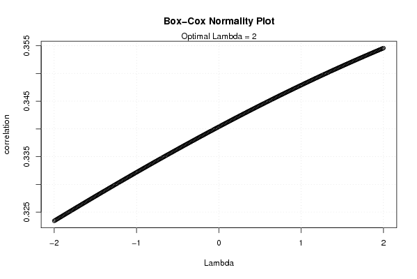
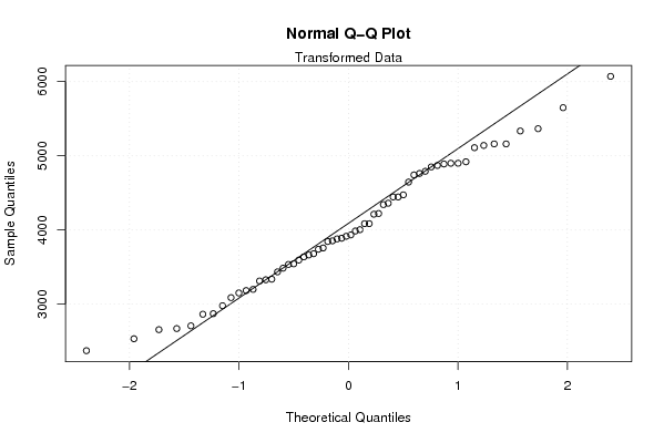
| Title produced by software | Box-Cox Normality Plot | ||||||||||||||||||||||||||||||||||||
| Date of computation | Sun, 23 Nov 2008 06:17:31 -0700 | ||||||||||||||||||||||||||||||||||||
| Cite this page as follows | Statistical Computations at FreeStatistics.org, Office for Research Development and Education, URL https://freestatistics.org/blog/index.php?v=date/2008/Nov/23/t12274462921g5zmuuf28u2wnh.htm/, Retrieved Sun, 19 May 2024 03:47:59 +0000 | ||||||||||||||||||||||||||||||||||||
| Statistical Computations at FreeStatistics.org, Office for Research Development and Education, URL https://freestatistics.org/blog/index.php?pk=25250, Retrieved Sun, 19 May 2024 03:47:59 +0000 | |||||||||||||||||||||||||||||||||||||
| QR Codes: | |||||||||||||||||||||||||||||||||||||
|
| |||||||||||||||||||||||||||||||||||||
| Original text written by user: | |||||||||||||||||||||||||||||||||||||
| IsPrivate? | No (this computation is public) | ||||||||||||||||||||||||||||||||||||
| User-defined keywords | |||||||||||||||||||||||||||||||||||||
| Estimated Impact | 164 | ||||||||||||||||||||||||||||||||||||
Tree of Dependent Computations | |||||||||||||||||||||||||||||||||||||
| Family? (F = Feedback message, R = changed R code, M = changed R Module, P = changed Parameters, D = changed Data) | |||||||||||||||||||||||||||||||||||||
| F [Box-Cox Linearity Plot] [various eda q3] [2008-11-10 14:09:04] [85134b6edb9973b9193450dd2306c65b] - RM D [Box-Cox Normality Plot] [Hercomputatie fee...] [2008-11-21 20:27:09] [deb3c14ac9e4607a6d84fc9d0e0e6cc2] - D [Box-Cox Normality Plot] [Q5] [2008-11-23 13:17:31] [541f63fa3157af9df10fc4d202b2a90b] [Current] | |||||||||||||||||||||||||||||||||||||
| Feedback Forum | |||||||||||||||||||||||||||||||||||||
Post a new message | |||||||||||||||||||||||||||||||||||||
Dataset | |||||||||||||||||||||||||||||||||||||
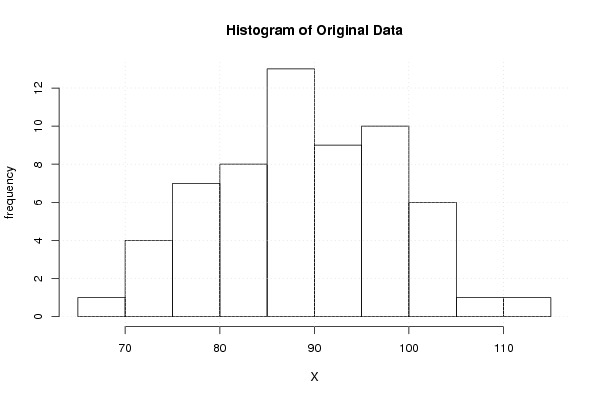
| Dataseries X: | |||||||||||||||||||||||||||||||||||||
81,6 84,1 88,1 85,3 82,9 84,8 71,2 68,9 94,3 97,6 85,6 91,9 75,8 79,8 99 88,5 86,7 97,9 94,3 72,9 91,8 93,2 86,5 98,9 77,2 79,4 90,4 81,4 85,8 103,6 73,6 75,7 99,2 88,7 94,6 98,7 84,2 87,7 103,3 88,2 93,4 106,3 73,1 78,6 101,6 101,4 98,5 99 89,5 83,5 97,4 87,8 90,4 101,6 80 81,7 96,4 110,2 101,1 89,3 | |||||||||||||||||||||||||||||||||||||
Tables (Output of Computation) | |||||||||||||||||||||||||||||||||||||
| |||||||||||||||||||||||||||||||||||||
Figures (Output of Computation) | |||||||||||||||||||||||||||||||||||||
Input Parameters & R Code | |||||||||||||||||||||||||||||||||||||
| Parameters (Session): | |||||||||||||||||||||||||||||||||||||
| Parameters (R input): | |||||||||||||||||||||||||||||||||||||
| R code (references can be found in the software module): | |||||||||||||||||||||||||||||||||||||
n <- length(x) | |||||||||||||||||||||||||||||||||||||