Free Statistics
of Irreproducible Research!
Description of Statistical Computation | |||||||||||||||||||||||||||||||||||||||||||||||||||||
|---|---|---|---|---|---|---|---|---|---|---|---|---|---|---|---|---|---|---|---|---|---|---|---|---|---|---|---|---|---|---|---|---|---|---|---|---|---|---|---|---|---|---|---|---|---|---|---|---|---|---|---|---|---|
| Author's title | |||||||||||||||||||||||||||||||||||||||||||||||||||||
| Author | *Unverified author* | ||||||||||||||||||||||||||||||||||||||||||||||||||||
| R Software Module | rwasp_edauni.wasp | ||||||||||||||||||||||||||||||||||||||||||||||||||||
| Title produced by software | Univariate Explorative Data Analysis | ||||||||||||||||||||||||||||||||||||||||||||||||||||
| Date of computation | Sat, 25 Oct 2008 08:07:21 -0600 | ||||||||||||||||||||||||||||||||||||||||||||||||||||
| Cite this page as follows | Statistical Computations at FreeStatistics.org, Office for Research Development and Education, URL https://freestatistics.org/blog/index.php?v=date/2008/Oct/25/t1224943729sxvzsshl2hjcqm1.htm/, Retrieved Wed, 15 May 2024 20:26:32 +0000 | ||||||||||||||||||||||||||||||||||||||||||||||||||||
| Statistical Computations at FreeStatistics.org, Office for Research Development and Education, URL https://freestatistics.org/blog/index.php?pk=18742, Retrieved Wed, 15 May 2024 20:26:32 +0000 | |||||||||||||||||||||||||||||||||||||||||||||||||||||
| QR Codes: | |||||||||||||||||||||||||||||||||||||||||||||||||||||
|
| |||||||||||||||||||||||||||||||||||||||||||||||||||||
| Original text written by user: | |||||||||||||||||||||||||||||||||||||||||||||||||||||
| IsPrivate? | No (this computation is public) | ||||||||||||||||||||||||||||||||||||||||||||||||||||
| User-defined keywords | Whisky | ||||||||||||||||||||||||||||||||||||||||||||||||||||
| Estimated Impact | 166 | ||||||||||||||||||||||||||||||||||||||||||||||||||||
Tree of Dependent Computations | |||||||||||||||||||||||||||||||||||||||||||||||||||||
| Family? (F = Feedback message, R = changed R code, M = changed R Module, P = changed Parameters, D = changed Data) | |||||||||||||||||||||||||||||||||||||||||||||||||||||
| F [Univariate Explorative Data Analysis] [Investigating dis...] [2007-10-22 19:45:25] [b9964c45117f7aac638ab9056d451faa] F D [Univariate Explorative Data Analysis] [investigating dis...] [2008-10-25 13:32:53] [5de5fb433ddcb9578e0fa830f795b7e9] - D [Univariate Explorative Data Analysis] [investigating dis...] [2008-10-25 14:07:21] [d8c5724db236abb5950452133b88474d] [Current] - D [Univariate Explorative Data Analysis] [Investigation val...] [2008-10-27 22:01:55] [74be16979710d4c4e7c6647856088456] - [Univariate Explorative Data Analysis] [Investigation val...] [2008-10-27 22:10:04] [74be16979710d4c4e7c6647856088456] | |||||||||||||||||||||||||||||||||||||||||||||||||||||
| Feedback Forum | |||||||||||||||||||||||||||||||||||||||||||||||||||||
Post a new message | |||||||||||||||||||||||||||||||||||||||||||||||||||||
Dataset | |||||||||||||||||||||||||||||||||||||||||||||||||||||
| Dataseries X: | |||||||||||||||||||||||||||||||||||||||||||||||||||||
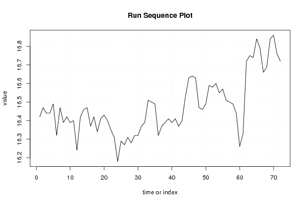
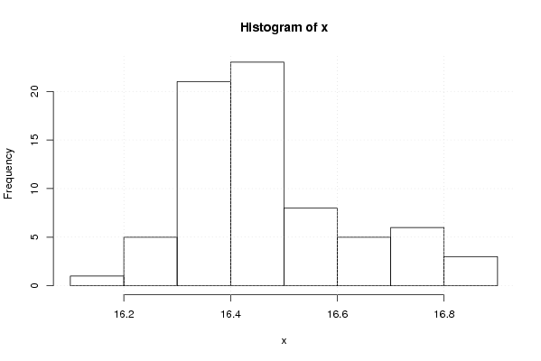
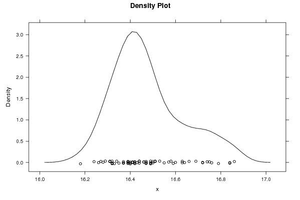
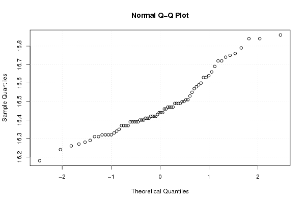
16,42 16,47 16,44 16,44 16,49 16,32 16,47 16,39 16,42 16,39 16,4 16,24 16,42 16,46 16,47 16,37 16,42 16,34 16,41 16,43 16,4 16,35 16,31 16,18 16,29 16,27 16,31 16,28 16,32 16,32 16,37 16,39 16,51 16,5 16,49 16,32 16,37 16,39 16,41 16,39 16,41 16,37 16,4 16,53 16,63 16,64 16,63 16,47 16,46 16,49 16,59 16,58 16,6 16,55 16,57 16,51 16,5 16,49 16,44 16,26 16,33 16,72 16,75 16,74 16,84 16,79 16,66 16,69 16,84 16,86 16,76 16,72 | |||||||||||||||||||||||||||||||||||||||||||||||||||||
Tables (Output of Computation) | |||||||||||||||||||||||||||||||||||||||||||||||||||||
| |||||||||||||||||||||||||||||||||||||||||||||||||||||
Figures (Output of Computation) | |||||||||||||||||||||||||||||||||||||||||||||||||||||
Input Parameters & R Code | |||||||||||||||||||||||||||||||||||||||||||||||||||||
| Parameters (Session): | |||||||||||||||||||||||||||||||||||||||||||||||||||||
| par1 = 0 ; par2 = 0 ; | |||||||||||||||||||||||||||||||||||||||||||||||||||||
| Parameters (R input): | |||||||||||||||||||||||||||||||||||||||||||||||||||||
| par1 = 0 ; par2 = 0 ; | |||||||||||||||||||||||||||||||||||||||||||||||||||||
| R code (references can be found in the software module): | |||||||||||||||||||||||||||||||||||||||||||||||||||||
par1 <- as.numeric(par1) | |||||||||||||||||||||||||||||||||||||||||||||||||||||