Free Statistics

of Irreproducible Research!

Author's title

Author*The author of this computation has been verified*
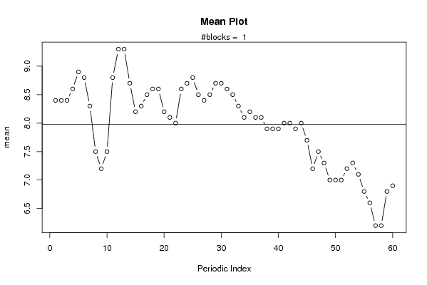
R Software Modulerwasp_meanplot.wasp
Title produced by softwareMean Plot
Date of computationWed, 29 Oct 2008 09:23:13 -0600
Cite this page as followsStatistical Computations at FreeStatistics.org, Office for Research Development and Education, URL https://freestatistics.org/blog/index.php?v=date/2008/Oct/29/t1225293886mq1lqtf6rn7omk5.htm/, Retrieved Sat, 18 May 2024 05:48:54 +0000
Statistical Computations at FreeStatistics.org, Office for Research Development and Education, URL https://freestatistics.org/blog/index.php?pk=19886, Retrieved Sat, 18 May 2024 05:48:54 +0000
QR Codes:

Original text written by user:
IsPrivate?No (this computation is public)
User-defined keywordsMean plot eigen datareeks
Estimated Impact183
Family? (F = Feedback message, R = changed R code, M = changed R Module, P = changed Parameters, D = changed Data)
F     [Mean Plot] [workshop 3] [2007-10-26 12:14:28] [e9ffc5de6f8a7be62f22b142b5b6b1a8]
F R PD    [Mean Plot] [Mean plot eigen d...] [2008-10-29 15:23:13] [f4b2017b314c03698059f43b95818e67] [Current]
F   P       [Mean Plot] [tt4] [2008-10-30 09:18:17] [a18c43c8b63fa6800a53bb187b9ddd45]
-   P         [Mean Plot] [asses] [2008-11-11 11:39:46] [74be16979710d4c4e7c6647856088456]
Feedback Forum
2008-11-10 20:27:08 [Nick Wuyts] [reply
De student gebruikt de techniek van het meanplot voor zijn eigen tijdreeks, wat correct is. Er wordt niet vermeld over wat deze tijdreeks gaat. Ook worden enige outliers niet verklaard.
Volgens mij is er een steeds terugkerende lichte stijging op te merken (grafiek mean plot), de eerste heeft plaats rond waarde 7 (x-as), de volgende bij 19, 23, 30 etc. Dit zou kunnen wijzen op seizoenaliteit.
De 2 grafieken notched boxplots periodic- en differenced periodic subseries zijn merkwaardig. Zij vertonen geen boxplotfiguurtjes met inkepingen, maar platte punten.

Post a new message
Dataseries X:
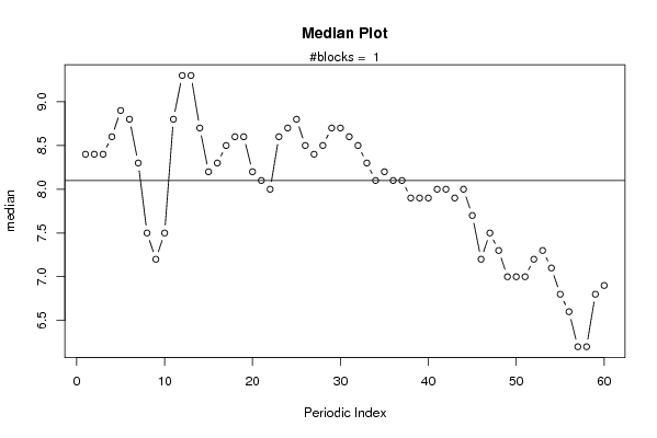
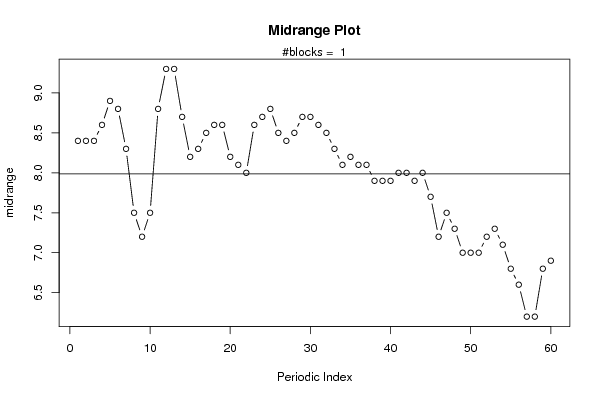
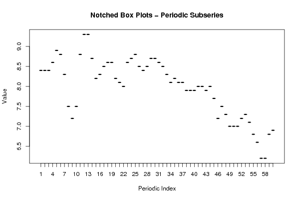
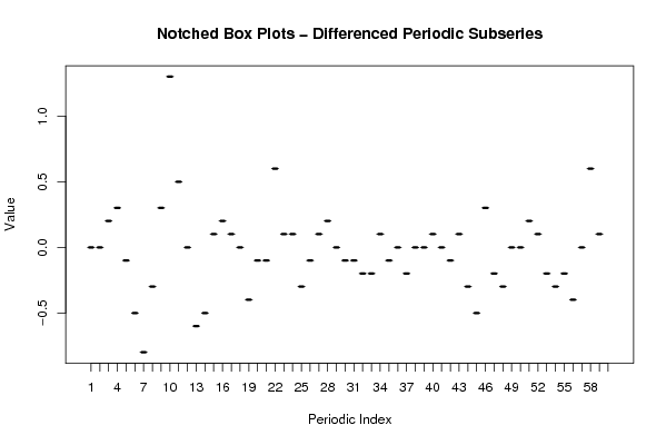
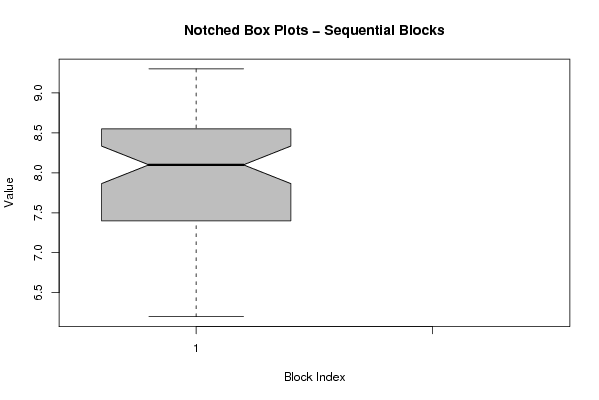
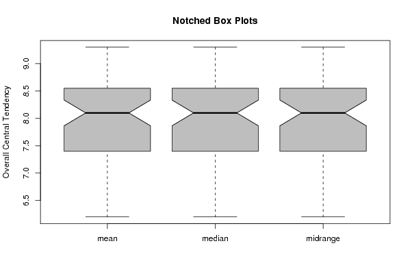
8.4
8.4
8.4
8.6
8.9
8.8
8.3
7.5
7.2
7.5
8.8
9.3
9.3
8.7
8.2
8.3
8.5
8.6
8.6
8.2
8.1
8
8.6
8.7
8.8
8.5
8.4
8.5
8.7
8.7
8.6
8.5
8.3
8.1
8.2
8.1
8.1
7.9
7.9
7.9
8
8
7.9
8
7.7
7.2
7.5
7.3
7
7
7
7.2
7.3
7.1
6.8
6.6
6.2
6.2
6.8
6.9


Summary of computational transaction
Raw Inputview raw input (R code)
Raw Outputview raw output of R engine
Computing time2 seconds
R Server'Gwilym Jenkins' @ 72.249.127.135

\begin{tabular}{lllllllll}
\hline
Summary of computational transaction \tabularnewline
Raw Input & view raw input (R code)  \tabularnewline
Raw Output & view raw output of R engine  \tabularnewline
Computing time & 2 seconds \tabularnewline
R Server & 'Gwilym Jenkins' @ 72.249.127.135 \tabularnewline
\hline
\end{tabular}
%Source: https://freestatistics.org/blog/index.php?pk=19886&T=0

[TABLE]
[ROW][C]Summary of computational transaction[/C][/ROW]
[ROW][C]Raw Input[/C][C]view raw input (R code) [/C][/ROW]
[ROW][C]Raw Output[/C][C]view raw output of R engine [/C][/ROW]
[ROW][C]Computing time[/C][C]2 seconds[/C][/ROW]
[ROW][C]R Server[/C][C]'Gwilym Jenkins' @ 72.249.127.135[/C][/ROW]
[/TABLE]
Source: https://freestatistics.org/blog/index.php?pk=19886&T=0

Globally Unique Identifier (entire table): ba.freestatistics.org/blog/index.php?pk=19886&T=0

As an alternative you can also use a QR Code:  

The GUIDs for individual cells are displayed in the table below:

Summary of computational transaction
Raw Inputview raw input (R code)
Raw Outputview raw output of R engine
Computing time2 seconds
R Server'Gwilym Jenkins' @ 72.249.127.135


Parameters (Session):
par1 = grey ;
Parameters (R input):
par1 = 60 ;
R code (references can be found in the software module):
par1 <- as.numeric(par1)
(n <- length(x))
(np <- floor(n / par1))
arr <- array(NA,dim=c(par1,np+1))
darr <- array(NA,dim=c(par1,np+1))
ari <- array(0,dim=par1)
dx <- diff(x)
j <- 0
for (i in 1:n)
{
j = j + 1
ari[j] = ari[j] + 1
arr[j,ari[j]] <- x[i]
darr[j,ari[j]] <- dx[i]
if (j == par1) j = 0
}
ari
arr
darr
arr.mean <- array(NA,dim=par1)
arr.median <- array(NA,dim=par1)
arr.midrange <- array(NA,dim=par1)
for (j in 1:par1)
{
arr.mean[j] <- mean(arr[j,],na.rm=TRUE)
arr.median[j] <- median(arr[j,],na.rm=TRUE)
arr.midrange[j] <- (quantile(arr[j,],0.75,na.rm=TRUE) + quantile(arr[j,],0.25,na.rm=TRUE)) / 2
}
overall.mean <- mean(x)
overall.median <- median(x)
overall.midrange <- (quantile(x,0.75) + quantile(x,0.25)) / 2
bitmap(file='plot1.png')
plot(arr.mean,type='b',ylab='mean',main='Mean Plot',xlab='Periodic Index')
mtext(paste('#blocks = ',np))
abline(overall.mean,0)
dev.off()
bitmap(file='plot2.png')
plot(arr.median,type='b',ylab='median',main='Median Plot',xlab='Periodic Index')
mtext(paste('#blocks = ',np))
abline(overall.median,0)
dev.off()
bitmap(file='plot3.png')
plot(arr.midrange,type='b',ylab='midrange',main='Midrange Plot',xlab='Periodic Index')
mtext(paste('#blocks = ',np))
abline(overall.midrange,0)
dev.off()
bitmap(file='plot4.png')
z <- data.frame(t(arr))
names(z) <- c(1:par1)
(boxplot(z,notch=TRUE,col='grey',xlab='Periodic Index',ylab='Value',main='Notched Box Plots - Periodic Subseries'))
dev.off()
bitmap(file='plot4b.png')
z <- data.frame(t(darr))
names(z) <- c(1:par1)
(boxplot(z,notch=TRUE,col='grey',xlab='Periodic Index',ylab='Value',main='Notched Box Plots - Differenced Periodic Subseries'))
dev.off()
bitmap(file='plot5.png')
z <- data.frame(arr)
names(z) <- c(1:np)
(boxplot(z,notch=TRUE,col='grey',xlab='Block Index',ylab='Value',main='Notched Box Plots - Sequential Blocks'))
dev.off()
bitmap(file='plot6.png')
z <- data.frame(cbind(arr.mean,arr.median,arr.midrange))
names(z) <- list('mean','median','midrange')
(boxplot(z,notch=TRUE,col='grey',ylab='Overall Central Tendency',main='Notched Box Plots'))
dev.off()