Free Statistics
of Irreproducible Research!
Description of Statistical Computation | |||||||||||||||||||||
|---|---|---|---|---|---|---|---|---|---|---|---|---|---|---|---|---|---|---|---|---|---|
| Author's title | |||||||||||||||||||||
| Author | *The author of this computation has been verified* | ||||||||||||||||||||
| R Software Module | rwasp_meanplot.wasp | ||||||||||||||||||||
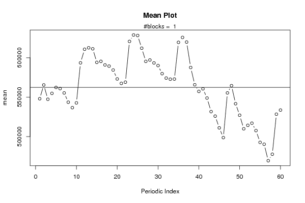
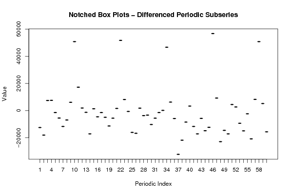
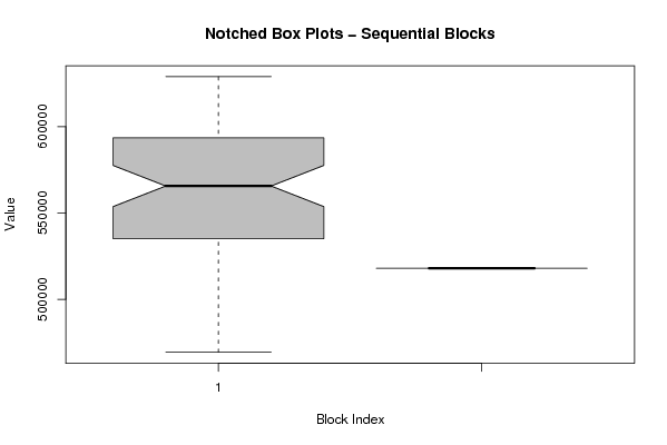
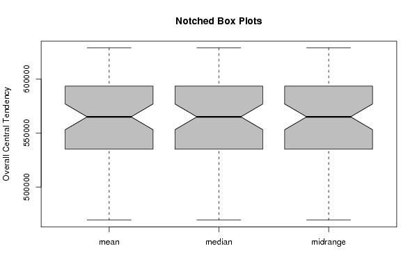
| Title produced by software | Mean Plot | ||||||||||||||||||||
| Date of computation | Wed, 29 Oct 2008 10:41:05 -0600 | ||||||||||||||||||||
| Cite this page as follows | Statistical Computations at FreeStatistics.org, Office for Research Development and Education, URL https://freestatistics.org/blog/index.php?v=date/2008/Oct/29/t1225298530m8q1dv2r5oze86x.htm/, Retrieved Fri, 17 May 2024 03:20:54 +0000 | ||||||||||||||||||||
| Statistical Computations at FreeStatistics.org, Office for Research Development and Education, URL https://freestatistics.org/blog/index.php?pk=19908, Retrieved Fri, 17 May 2024 03:20:54 +0000 | |||||||||||||||||||||
| QR Codes: | |||||||||||||||||||||
|
| |||||||||||||||||||||
| Original text written by user: | |||||||||||||||||||||
| IsPrivate? | No (this computation is public) | ||||||||||||||||||||
| User-defined keywords | |||||||||||||||||||||
| Estimated Impact | 148 | ||||||||||||||||||||
Tree of Dependent Computations | |||||||||||||||||||||
| Family? (F = Feedback message, R = changed R code, M = changed R Module, P = changed Parameters, D = changed Data) | |||||||||||||||||||||
| F [Univariate Data Series] [Niet werkende wer...] [2008-10-13 17:21:04] [91d2608132ba5d00ecce3524d8276757] F RMP [Mean Plot] [Taak 5, Mean plot...] [2008-10-29 16:41:05] [5e9e099b83e50415d7642e10d74756e4] [Current] - P [Mean Plot] [Taak 5] [2008-11-06 19:12:14] [ed2ba3b6182103c15c0ab511ae4e6284] | |||||||||||||||||||||
| Feedback Forum | |||||||||||||||||||||
Post a new message | |||||||||||||||||||||
Dataset | |||||||||||||||||||||
| Dataseries X: | |||||||||||||||||||||
577992 565464 547344 554788 562325 560854 555332 543599 536662 542722 593530 610763 612613 611324 594167 595454 590865 589379 584428 573100 567456 569028 620735 628884 628232 612117 595404 597141 593408 590072 579799 574205 572775 572942 619567 625809 619916 587625 565742 557274 560576 548854 531673 525919 511038 498662 555362 564591 541657 527070 509846 514258 516922 507561 492622 490243 469357 477580 528379 533590 517945 | |||||||||||||||||||||
Tables (Output of Computation) | |||||||||||||||||||||
| |||||||||||||||||||||
Figures (Output of Computation) | |||||||||||||||||||||
Input Parameters & R Code | |||||||||||||||||||||
| Parameters (Session): | |||||||||||||||||||||
| par1 = 60 ; | |||||||||||||||||||||
| Parameters (R input): | |||||||||||||||||||||
| par1 = 60 ; | |||||||||||||||||||||
| R code (references can be found in the software module): | |||||||||||||||||||||
par1 <- as.numeric(par1) | |||||||||||||||||||||