Free Statistics
of Irreproducible Research!
Description of Statistical Computation | |||||||||||||||||||||
|---|---|---|---|---|---|---|---|---|---|---|---|---|---|---|---|---|---|---|---|---|---|
| Author's title | |||||||||||||||||||||
| Author | *The author of this computation has been verified* | ||||||||||||||||||||
| R Software Module | rwasp_meanplot.wasp | ||||||||||||||||||||
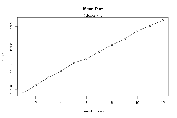
| Title produced by software | Mean Plot | ||||||||||||||||||||
| Date of computation | Wed, 29 Oct 2008 12:45:02 -0600 | ||||||||||||||||||||
| Cite this page as follows | Statistical Computations at FreeStatistics.org, Office for Research Development and Education, URL https://freestatistics.org/blog/index.php?v=date/2008/Oct/29/t1225305970v5c3pk6xi4w29r8.htm/, Retrieved Fri, 17 May 2024 04:14:40 +0000 | ||||||||||||||||||||
| Statistical Computations at FreeStatistics.org, Office for Research Development and Education, URL https://freestatistics.org/blog/index.php?pk=19936, Retrieved Fri, 17 May 2024 04:14:40 +0000 | |||||||||||||||||||||
| QR Codes: | |||||||||||||||||||||
|
| |||||||||||||||||||||
| Original text written by user: | |||||||||||||||||||||
| IsPrivate? | No (this computation is public) | ||||||||||||||||||||
| User-defined keywords | |||||||||||||||||||||
| Estimated Impact | 147 | ||||||||||||||||||||
Tree of Dependent Computations | |||||||||||||||||||||
| Family? (F = Feedback message, R = changed R code, M = changed R Module, P = changed Parameters, D = changed Data) | |||||||||||||||||||||
| F [Mean Plot] [workshop 3] [2007-10-26 12:14:28] [e9ffc5de6f8a7be62f22b142b5b6b1a8] F D [Mean Plot] [Hypothesis Testin...] [2008-10-29 16:51:46] [a57f5cc542637534b8bb5bcb4d37eab1] F D [Mean Plot] [Hypothesis Testin...] [2008-10-29 18:45:02] [0f30549460cf4ec26d9cf94b1fcf7789] [Current] F D [Mean Plot] [Hypothesis Testin...] [2008-10-29 18:46:57] [a57f5cc542637534b8bb5bcb4d37eab1] | |||||||||||||||||||||
| Feedback Forum | |||||||||||||||||||||
Post a new message | |||||||||||||||||||||
Dataset | |||||||||||||||||||||
| Dataseries X: | |||||||||||||||||||||
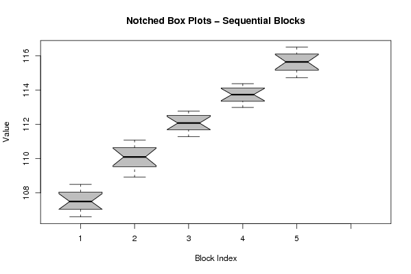
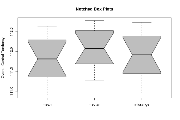
106,60 106,80 107,00 107,10 107,30 107,40 107,60 107,70 107,90 108,20 108,30 108,50 108,92 109,23 109,41 109,65 109,91 110,01 110,20 110,49 110,57 110,72 110,94 111,09 111,28 111,41 111,62 111,76 111,89 112,04 112,12 112,30 112,47 112,59 112,78 112,73 112,99 113,10 113,33 113,38 113,68 113,65 113,81 113,88 114,02 114,25 114,28 114,38 114,73 114,97 115,05 115,29 115,37 115,54 115,76 115,92 116,02 116,21 116,26 116,51 | |||||||||||||||||||||
Tables (Output of Computation) | |||||||||||||||||||||
| |||||||||||||||||||||
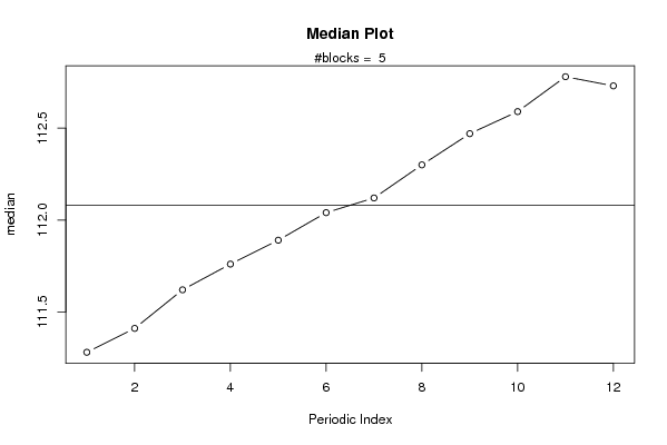
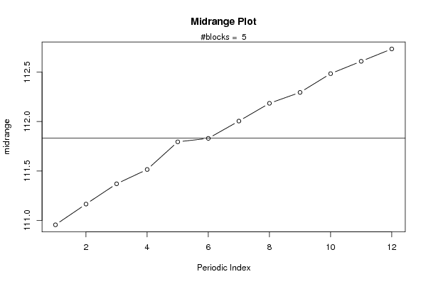
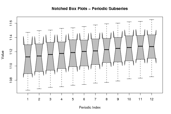
Figures (Output of Computation) | |||||||||||||||||||||
Input Parameters & R Code | |||||||||||||||||||||
| Parameters (Session): | |||||||||||||||||||||
| par1 = 12 ; | |||||||||||||||||||||
| Parameters (R input): | |||||||||||||||||||||
| par1 = 12 ; | |||||||||||||||||||||
| R code (references can be found in the software module): | |||||||||||||||||||||
par1 <- as.numeric(par1) | |||||||||||||||||||||