Free Statistics
of Irreproducible Research!
Description of Statistical Computation | |||||||||||||||||||||
|---|---|---|---|---|---|---|---|---|---|---|---|---|---|---|---|---|---|---|---|---|---|
| Author's title | |||||||||||||||||||||
| Author | *Unverified author* | ||||||||||||||||||||
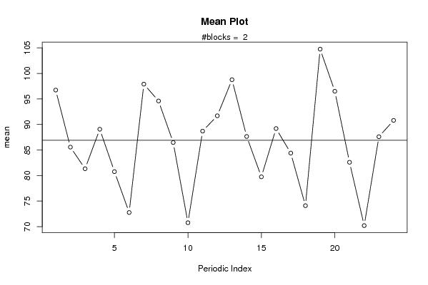
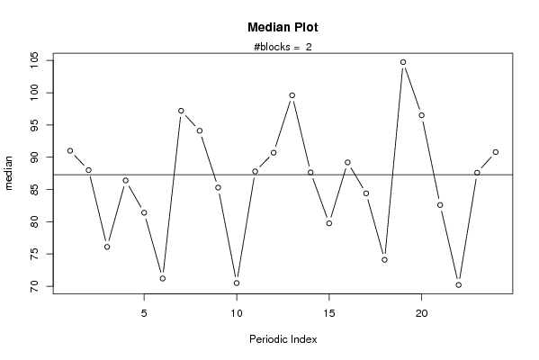
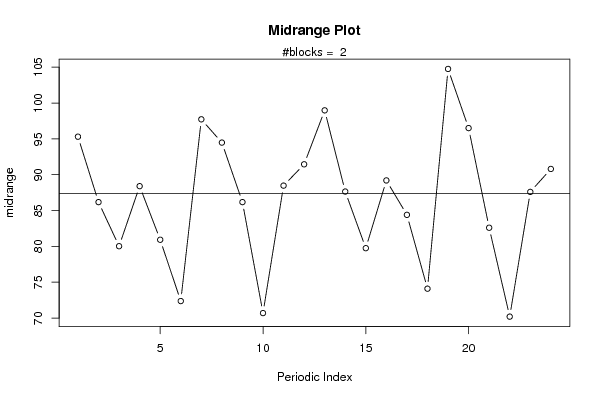
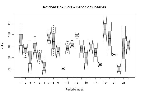
| R Software Module | rwasp_meanplot.wasp | ||||||||||||||||||||
| Title produced by software | Mean Plot | ||||||||||||||||||||
| Date of computation | Thu, 30 Oct 2008 08:52:35 -0600 | ||||||||||||||||||||
| Cite this page as follows | Statistical Computations at FreeStatistics.org, Office for Research Development and Education, URL https://freestatistics.org/blog/index.php?v=date/2008/Oct/30/t1225378389sxvq8s5hmpwxlvp.htm/, Retrieved Fri, 17 May 2024 03:07:53 +0000 | ||||||||||||||||||||
| Statistical Computations at FreeStatistics.org, Office for Research Development and Education, URL https://freestatistics.org/blog/index.php?pk=20071, Retrieved Fri, 17 May 2024 03:07:53 +0000 | |||||||||||||||||||||
| QR Codes: | |||||||||||||||||||||
|
| |||||||||||||||||||||
| Original text written by user: | |||||||||||||||||||||
| IsPrivate? | No (this computation is public) | ||||||||||||||||||||
| User-defined keywords | |||||||||||||||||||||
| Estimated Impact | 176 | ||||||||||||||||||||
Tree of Dependent Computations | |||||||||||||||||||||
| Family? (F = Feedback message, R = changed R code, M = changed R Module, P = changed Parameters, D = changed Data) | |||||||||||||||||||||
| F [Mean Plot] [q2 mean plot] [2008-10-30 14:52:35] [4940af498c7c54f3992f17142bd40069] [Current] - PD [Mean Plot] [q2 mean plot goed] [2008-10-30 14:56:11] [85134b6edb9973b9193450dd2306c65b] F D [Mean Plot] [q3 mean plot] [2008-10-30 15:32:57] [85134b6edb9973b9193450dd2306c65b] F RMPD [Bootstrap Plot - Central Tendency] [q4 blocked bootstrap] [2008-10-30 15:47:17] [85134b6edb9973b9193450dd2306c65b] F RM D [Notched Boxplots] [task 2 notched bo...] [2008-10-30 17:01:13] [85134b6edb9973b9193450dd2306c65b] F R PD [Notched Boxplots] [task 3 notched bo...] [2008-10-30 17:22:47] [85134b6edb9973b9193450dd2306c65b] F RMPD [Mean Plot] [taak 5 mean plot] [2008-10-30 18:39:42] [85134b6edb9973b9193450dd2306c65b] - P [Mean Plot] [verbetering taak 5] [2008-11-09 13:07:12] [85134b6edb9973b9193450dd2306c65b] - P [Mean Plot] [Oplossing Taak 5] [2008-11-11 13:29:58] [f9b9e85820b2a54b20380c3265aca831] - PD [Mean Plot] [verbetering q2] [2008-11-09 12:28:20] [85134b6edb9973b9193450dd2306c65b] | |||||||||||||||||||||
| Feedback Forum | |||||||||||||||||||||
Post a new message | |||||||||||||||||||||
Dataset | |||||||||||||||||||||
| Dataseries X: | |||||||||||||||||||||
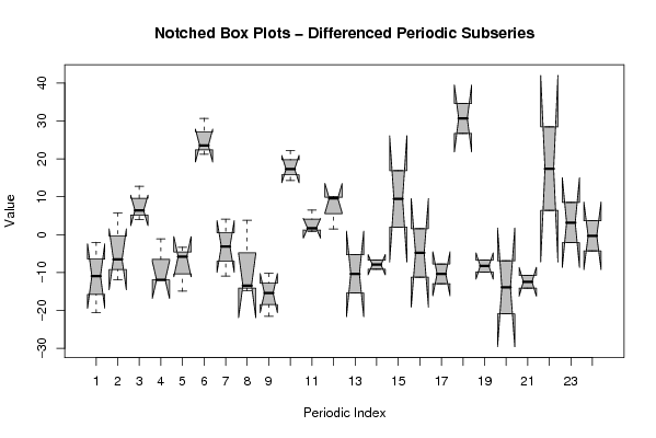
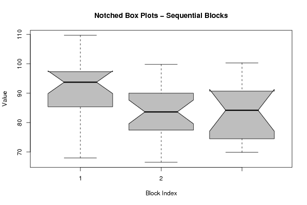
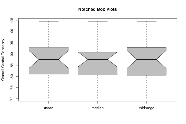
109,20 88,60 94,30 98,30 86,40 80,60 104,10 108,20 93,40 71,90 94,10 94,90 96,40 91,10 84,40 86,40 88,00 75,10 109,70 103,00 82,10 68,00 96,40 94,30 90,00 88,00 76,10 82,50 81,40 66,50 97,20 94,10 80,70 70,50 87,80 89,50 99,60 84,20 75,10 92,00 80,80 73,10 99,80 90,00 83,10 72,40 78,80 87,30 91,00 80,10 73,60 86,40 74,50 71,20 92,40 81,50 85,30 69,90 84,20 90,70 100,30 | |||||||||||||||||||||
Tables (Output of Computation) | |||||||||||||||||||||
| |||||||||||||||||||||
Figures (Output of Computation) | |||||||||||||||||||||
Input Parameters & R Code | |||||||||||||||||||||
| Parameters (Session): | |||||||||||||||||||||
| Parameters (R input): | |||||||||||||||||||||
| par1 = 24 ; | |||||||||||||||||||||
| R code (references can be found in the software module): | |||||||||||||||||||||
par1 <- as.numeric(par1) | |||||||||||||||||||||